


(C) 2012 Qinfeng Guo. This is an open access article distributed under the terms of the Creative Commons Attribution License 3.0 (CC-BY), which permits unrestricted use, distribution, and reproduction in any medium, provided the original author and source are credited.
For reference, use of the paginated PDF or printed version of this article is recommended.
Previous studies on alien species establishment in the United States and around the world have drastically improved our understanding of the patterns of species naturalization, biological invasions, and underlying mechanisms. Meanwhile, relevant new data have been added and the data quality has significantly increased along with the consistency of related concepts and terminology that are being developed. Here using new and/or improved data on the native and exotic plant richness and many socioeconomic and physical variables at the state level in the United States, we attempt to test whether previously discovered patterns still hold, particularly how native and exotic species are related and what are the dominant factors controlling the plant naturalization. We found that, while the number of native species is largely controlled by natural factors such as area and temperature, exotic species and exotic fraction are predominantly influenced by social factors such as human population. When domestically introduced species were included, several aspects in earlier findings were somewhat altered and additional insights regarding the mechanisms of naturalization could be achieved. With increased data availability, however, a greater challenge ahead appears to be how many and which variables to included in analyses.
Native species diversity, domestic exotics, spatial correlation, species richness, state-level analysis
In the past decades, studies on the species naturalizations and invasions in the United States and around the world have drastically improved our understanding of the patterns and underlying mechanisms (e.g.,
On average, in the 48 conterminous US states, about 25% of naturalized plant species are domestically introduced from other states, which significantly increased the exotic richness but simultaneously decreased the earlier reported native richness in each state (
At the state-level, previous studies have examined and found significant effects of native richness, area, latitude, elevation, human population, the time since admission to the Union, and year of publication on the exotic species richness (or exotic fraction) across the United States (e.g.,
Results from multiple regression analyses showing the relationships between selected land-cover types and the corrected richness of native (a) and exotic (b) vascular plants and the exotic fraction (c) in the 48 conterminous US states (bold-faced P-values highlight the significant relationships). Temperature and precipitation represent mean annual temperature (ºC) and mean annual precipitation (cm), respectively. Here, exotic fraction was angular transformed, native and exotic richness, population size, years in the Union, and the number of ecoregions were log transformed, and the rest (mostly related to area) were square-root (sqrt) transformed before analyses.
| Native richness | Exotic richness | Exotic fraction | ||||||||
|---|---|---|---|---|---|---|---|---|---|---|
| Source | df | F-value | r2 | P | F-value | r2 | P | F-value | r2 | P |
| Model | 11 | 42.83 | 0.929 | <.0001 | 19.62 | 0.857 | <.0001 | 19.75 | 0.858 | <.0001 |
| Error | 36 | |||||||||
| Corrected total | 47 | |||||||||
| Variable | df | Parameter Estimate | t-value | P | Parameter Estimate | t-value | P | Parameter Estimate | t-value | P |
|---|---|---|---|---|---|---|---|---|---|---|
| Intercept | 1 | 2.58451 | 8.83 | <.0001 | 1.45469 | 1.61 | 0.116 | 3.29584 | 3.74 | 0.001 |
| Exotics | 1 | 0.04626 | .50 | 0.621 | -- | -- | -- | -- | -- | -- |
| Natives | 1 | -- | -- | -- | 0.14878 | 0.50 | 0.621 | -- | -- | -- |
| Land area (km2) | 1 | 0.02926 | 7.05 | <.0001 | -0.01633 | -1.46 | 0.152 | -0.00575 | -1.53 | 0.024 |
| Population size | 1 | 0.08528 | 2.28 | 0.029 | 0.21673 | 3.50 | 0.001 | 0.27662 | 4.57 | 0.0001 |
| Temperature (ºC) | 1 | 0.0767 | 6.07 | <.0001 | -0.06969 | -0.01 | 0.993 | -0.05032 | -1.66 | 0.105 |
| Precipitation (cm) | 1 | -0.00146 | -0.44 | 0.661 | -0.00221 | 0.37 | 0.711 | 0.00578 | 1.00 | 0.325 |
| Developed area (km2) | 1 | -0.00072 | -0.86 | 0.396 | -0.002 | 1.35 | 0.184 | 0.00104 | 0.72 | 0.474 |
| Cropland (km2) | 1 | -0.00165 | -7.46 | <.0001 | -0.00083 | -1.34 | 0.188 | -0.00176 | -2.92 | 0.006 |
| Forest (km2) | 1 | -0.0004 | -1.56 | 0.129 | 0.00073 | 1.58 | 0.124 | 0.000269 | 0.60 | 0.554 |
| Pasture/rangeland (km2) | 1 | -0.00042 | -1.66 | 0.105 | 0.00052 | 1.13 | 0.266 | 0.000642 | 1.42 | 0.164 |
| Years in Union | 1 | 0.06128 | 0.55 | 0.585 | 0.44498 | 2.39 | 0.022 | 0.32045 | 1.76 | 0.087 |
| No. Ecoregions | 1 | 0.11397 | 2.24 | 0.032 | -0.05242 | -0.54 | 0.593 | -0.01805 | -0.19 | 0.850 |
Here we follow the definition of naturalized plant species by
To examine the naturalization patterns related to geography (relative locations of each state), we made a simple comparison between border and interior states. The states with large water (i.e., oceans and the Great Lakes) were defined as border states and the rest as interior states. To examine the possible effects of selected social, economical, and physical variables on the naturalization patterns across the 48 conterminous US states, we related the number of native and exotic species and the exotic fraction to the human population, years since joining the Union, climate condition, the area, land cover types (below), and the number of eco-regions of each state (
The climate data (i.e., mean annual temperature, mean annual precipitation) for each state were obtained from http://www.cdc.noaa.gov/data/usclimate/ (1971-2000) and land cover data from http://www.allcountries.org/uscensus/ (1997). For the land cover data for each state, “developed area” includes urban and built-up areas such as highways, roads, cemeteries, airports, golf courses, landfills, small parks and other transportation facilities. “Cropland” includes both cultivated and non-cultivated lands such as hay fields and horticultural cropland. “Forestland” also includes land stocked by single-stemmed woody species, land of natural regeneration of tree cover, and land not currently developed for non-forest use. “Pastureland/Rangeland” includes land managed primarily for the production of introduced forage plants for livestock grazing and grasslands, savannas, many wetlands, some deserts, and tundra with climax or potential vegetation composed principally of native grasses, forbs or short shrubs suitable for grazing and browsing, and introduced forage species that are managed like rangeland species.
To analyze spatial autocorrelation for all selected variables, we calculated geodesic distances using the latitudinal and longitudinal data based on the center-point of each state. To examine the relative contribution of spatial autocorrelation, we applied and compared the results from both the ordinary-least-squares (OLS) estimation and spatial autoregression analyses (SAR). These two and the PCA analyses were performed using SAM (Spatial Analysis in Macroecology) (
In contrast to previously reported significant relationship between native and exotic species richness estimated based on the US boundary, using the corrected values (i.e., species truly native or exotic to each of the 48 states, rather than to the entire continental US), the relationship became non-significant (Fig. 1). The states with higher foreign exotic richness or fraction also had higher domestic exotic species richness or fraction (r2 = 0.83, p < 0.0001).
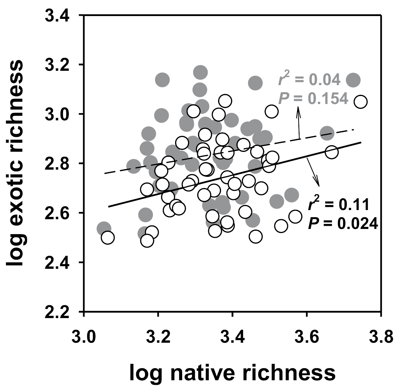
An example showing how the improved data of native vs. exotic species had altered previously described patterns of species naturalization in the United States. Using corrected values (i.e., species truly native or exotic to each of the 48 states, rather than to the entire continental United States), the relationship between native and exotic species richness became non-significant as indicated by the solid dots and dashed regression line. This result is in direct contrast with the previously reported significant relationship (open circles and solid regression line).
Analyses using the improved naturalized (Kartesz’s “exotic”) and native richness data across the 48 continental US states showed geographic (isolation) effects; i.e., although there was no difference in native richness between the border (coastal) states (with isolation on part of their borders) and interior states, the former had higher exotic richness and fractions than the latter (Fig. 2a). The exotic fraction decreased with state area but the declining rate was significantly higher for the interior states than for the border states (Fig. 2b; t = 3.79, P < 0.001). The top five states in the conterminous continental United States with the highest exotic fractions were all border states with rather small areas such as Massachusetts (84%), New York (71%), Pennsylvania (61%), Connecticut (60%), and Maine (55%) in the Northeast; whereas the ones with the lowest exotic fractions were the ones in the relatively dry and interior areas such as Arizona (13%), Nevada (13%), New Mexico (13%), Wyoming (16%), and Colorado (17%). In addition, our data show that the border states also have higher proportions of domestic exotics (i.e., domestic exotics/all exotics = 22%) than the interior states (15%; chi-square test, df = 1, P < 0.001).
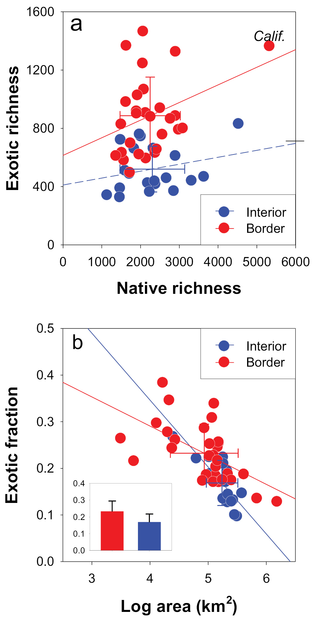
An example of geographical effects on the native and exotics richness in the conterminous continental United States. There was no significant difference in native richness between the border and interior states of the US but the border states showed significantly higher exotic richness and fraction than the interior states (t - test, P < 0.05). The exotic fraction decreased with state area and the interior states showed a greater decline. Here, natives and exotics were estimated using states own borders (bi-directional bars = SD).
Native richness was positively related to land area, temperature, human population size, and the number of ecoregions (as a measure of habitat diversity), but negatively related to the area of crop lands. By contrast, exotic species and exotic fraction were predominantly influenced by social factors (i.e., human population size). Exotic richness was also positively related to the number of years since joining the Union, and exotic fraction was also negatively affected by land area (
Results from PCA that extract orthogonal axes depicted a strong correlation structure (collinearity) among the selected state variables for the 48 conterminous continental US states. Several independent variables such as the number of ecoregions, human population size, pasture/rangeland, and urban area were positively related to each other and related to the response variable, native richness, along the first (horizontal) axis. Independent variables such as years in the Union and human population size were also positively related to each other and related to the exotic richness and exotic fraction (Fig. 3). The first component principal accounted for 37% of the total variance and the first two components (out of 13) accounted for 64% of the total variance. All variables except human population size were strongly correlated over space, but at different distances (Fig. S1). The state land area showed positive autocorrelations over the shortest distances and the number of eco-regions showed positive autocorrelations over the smallest distances, with other variables at intermediate distances. Interestingly, the exotic richness (and exotic fraction) exhibited significant positive spatial autocorrelation at a larger distance than native richness, suggesting greater homogenization (or similarity) in terms of species exotic floras across the 48 states than that in native floras (see also
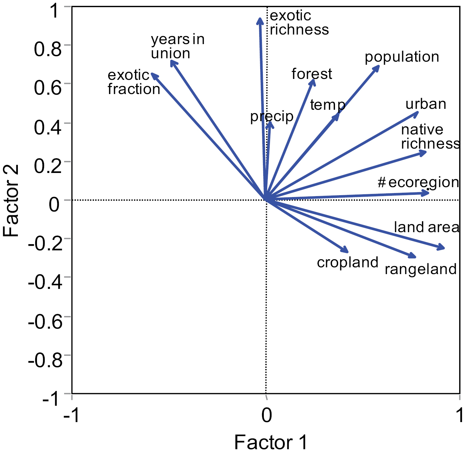
Results from Principal Component Analysis (PCA) that extracts orthogonal axes and shows the two-dimensional (PC1 and PC2) correlation structure among the selected state variables for the 48 conterminous continental US states. Here, “temp” represents temperature (ºC) and “precip” represents precipitation (cm).
To test the relative strength of spatial autocorrelation, which was measured based on the geodesic distances among the 48 states, we performed ordinary-least-squares (OLS) estimation and spatial autoregression analyses (SAR) that took both predictor variables and space (autocorrelation) into account. We then compared the results through both approaches. AICc values indicated that OLS (ordinary least squares multiple regression analysis) produced the best fitted models for native and exotic species richness and for exotic fraction (Table S1), despite the contributions from spatial autocorrelation in certain variables.
DiscussionIn agreement with several previous studies (
The border states are partly isolated from other interior states therefore should lose accessibility by some domestic exotics, but should have greater accessibility by foreign exotics through proportionally more and larger international airports and sea ports and earlier encounter of foreign sources of propagules (
While the number of native species is related to both natural and social variables, exotic richness and fraction are predominately influenced by human factors (see also
Two major issues deserve attention. First, it would be reasonable to argue that at least some of the differences in previously described patterns of species invasion or naturalization even from the same focal habitat or area stem either from inconsistent definition or inconsistent practice in regarding how to “correctly” count ‘exotics’. As
Second, increased data availability often leads to data dependency over space, time, or both, thus to violation of the assumptions of many statistical tests. It is still not clear whether, and to what extent, spatial or temporal autocorrelation and collinearity contribute to the inconsistency in earlier studies. In our particular case, spatial autoregressions confirm the results from multiple regressions and increase confidence in data interpretation. The OLS and SAR gave consistent results (Table S1), suggesting that the explanatory variables are also spatially autocorrelated (see Fig. S1). Thus, removing any autocorrelation among the explanatory variables would also remove most of the explanatory power of the explanatory variables. Unlike the native or exotic richness and exotic fraction, the residuals of most variables do not exhibit spatial autocorrelations (V. Jarosik, Personal Communications; see also
The multiple regressions confirm both positive effects of human population size on exotic species richness and exotic fraction, in the United States. Collinearity seems a greater statistical challenge than spatial autocorrelation. However, neither collinearity nor spatial autocorrelation seem to affect the overall results in this particular case. Nevertheless, knowing how the selected variables are spatially or temporally correlated might be informative, as they could affect the response variable interactively. When strong collinearity is detected, significantly reducing the number of variables would be an easy fix for collinearity but, at the same time, information and insights may be lost when ecological processes are influenced by additional factors than those selected. Further, adding more variables offers potentially more hypotheses and tests, and more detailed interpretations.
In summary, using newly added and improved data provides new insights regarding the plant naturalization mechanisms across the United States. All previously used independent variables at state-level analyses such human population, area, were also found significantly related to native and exotic plant richness. Yet, when additional variables were added, we found more variables that were significantly related to native and exotic richness and exotic fraction. Also, in this particular study at the state level, different statistical methods adopted here produced remarkably similar results regardless spatial correlation. However, a greater challenge ahead is how to properly handle greater numbers of variables with increased data availability, and caution is needed when dealing with data at other spatial scales (e.g., county-level).
We thank J.H. Brown, B. Cade, M. Davis, J. Falcone, D. Hooper, P. Hulme, V. Jarošík, K. Klepzig, J. Lepš, S. Norman, M. Palmer, R. Ricklefs, and J. Togerson for insightful comments on various versions of the manuscript; S. Creed, J. Kartesz, R. Moe, M. Nishino for their help with data compilation.
A sample of comparative results from the ordinary-least-squares (OLS) estimation and spatial autoregression analyses (SAR). Here we examined the effect of land area (km2) and its spatial autocorrelation (i.e., “space”) on exotic fraction, and native richness, and exotic richness. SAR on other variables showed very similar results in terms of the role of spatial autocorrelation (not shown).
| Native richness (log10) | Exotic richness (log10) | Exotic fraction | ||||
|---|---|---|---|---|---|---|
| AICc | AICc | AICc | ||||
| OLS | ||||||
| r2 | 0.416 | -73.099 | 0.071 | -28.398 | 0.466 | -42.580 |
| Constant(t) | 64.959*** | 47.284*** | -4.880** | |||
| Land area (t) | 5.286** | -0.536 | -3.252* | |||
| SAR | ||||||
| Land area (r2) | 0.416 | -73.099 | 0.037 | -26.652 | 0.386 | -35.868 |
| Land area + space (r2) | 0.449 | -75.884 | 0.058 | -7.704 | 0.406 | -37.466 |
* P < 0.01, ** P < 0.001, *** P < 0.0001.
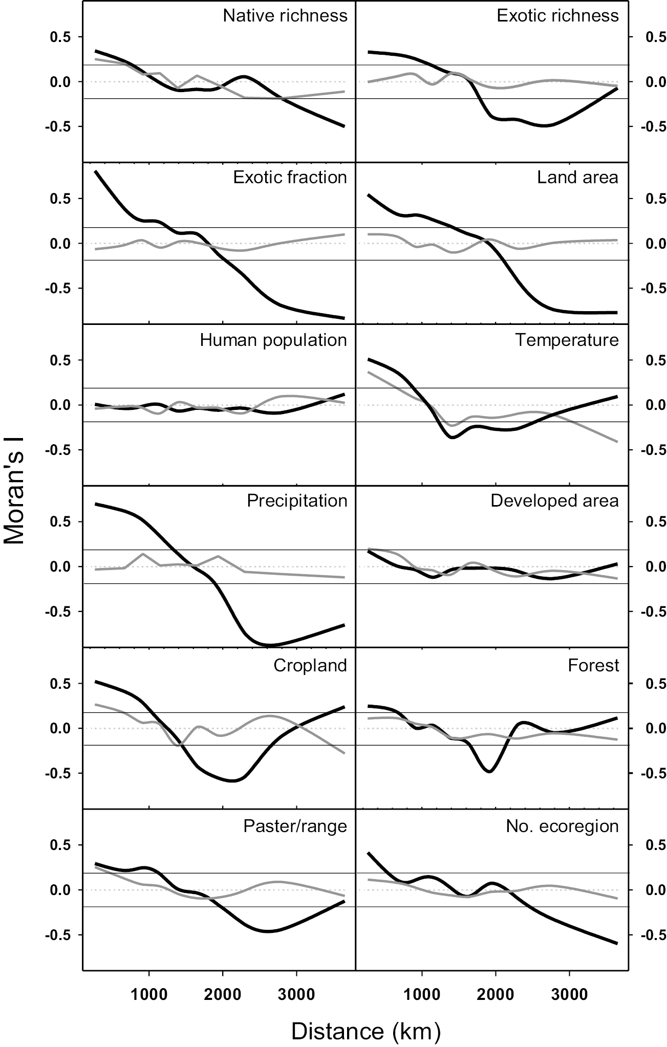
Spatial autocorrelation coefficient (Moran’s I) of species richness, exotic fraction, and other state variables (black line) and their residuals (gray lines) across the 48 conterminous continental US states. The data points above and upper or below the lower horizontal lines in each panel indicate significant spatial autocorrelations based on randomization (i.e., P < 0.05), using the Monte Carlo randomized data (distances; 200 replicates). For most variables, residuals do not show spatial autocorrelation (see