NeoBiota 14: 47–66, doi: 10.3897/neobiota.14.3273
Does residence time affect responses of alien species richness to environmental and spatial processes?
Matteo Dainese 1, Livio Poldini 2
1 Department of Land and Agroforest Environments, University of Padova, Viale dell’Università 16, I-35020 Legnaro, Padova, Italy
2 Department of Life Sciences, University of Trieste, via L. Giorgieri 10, I-34127 Trieste, Italy

Corresponding author: Matteo Dainese (matteo.dainese@unipd.it)

Academic editor: Ingolf Kühn

received 23 April 2012 | accepted 22 June 2012 | Published 22 August 2012


(C) 2012 Matteo Dainese. This is an open access article distributed under the terms of the Creative Commons Attribution License 3.0 (CC-BY), which permits unrestricted use, distribution, and reproduction in any medium, provided the original author and source are credited.


For reference, use of the paginated PDF or printed version of this article is recommended.

Abstract

One of the most robust emerging generalisations in invasion biology is that the probability of invasion increases with the time since introduction (residence time). We analysed the spatial distribution of alien vascular plant species in a region of north-eastern Italy to understand the influence of residence time on patterns of alien species richness. Neophytes were grouped according to three periods of arrival in the study region (1500–1800, 1800–1900, and > 1900). We applied multiple regression (spatial and non-spatial) with hierarchical partitioning to determine the influence of climate and human pressure on species richness within the groups. We also applied variation partitioning to evaluate the relative importance of environmental and spatial processes. Temperature mainly influenced groups with species having a longer residence time, while human pressure influenced the more recently introduced species, although its influence remained significant in all groups.Partial regression analyses showed that most of the variation explained by the models is attributable to spatially structured environmental variation, while environment and space had small independent effects. However, effects independent of environment decreased, and spatially independent effects increased, from older to the more recent neophytes. Our data illustrate that the distribution of alien species richness for species that arrived recently is related to propagule pressure, availability of novel niches created by human activity, and neutral-based (dispersal limitation) processes, while climate filtering plays a key role in the distribution of species that arrived earlier. This study highlights the importance of residence time, spatial structure, and environmental conditions in the patterns of alien species richness and for a better understanding of its geographical variation.

Keywords

Climate, dispersal limitation, energy, environmental filtering, human pressure, land-use, niche-based processes, propagule pressure

Introduction

Understanding the factors that determine the spatial distribution of exotic species is a primary objective of invasion ecology (Marini et al. 2009, de Albuquerque et al. 2011a, 2011b). Many factors have been postulated to influence invasiveness (the extent to which an introduced species is able to overcome various biotic and abiotic barriers, establish, proliferate, and disperse in a new environment) (Wilson et al. 2007).

Stochastic factors, including initial inoculum size, residence time, propagule pressure, and chance events (Richardson and Pyšek 2006), as well as, post introduction dispersal by human agency (Hodkinson and Thompson 1997, Kowarik 2003) are crucial for determining whether (or when) a species will invade. One of the most robust emerging generalisations in invasion biology is that the probability of invasion increases with the time since introduction (‘residence time’). Residence time integrates a suite of factors (some directly affecting propagule pressure) that potentially affect the success of an alien species: the longer the species is present in the region, the higher the likelihood that more propagules are spread, and the probability of founding new populations increases (Rejmánek et al. 2005, Richardson and Pyšek 2006). The positive relationship between residence time and current distribution of alien species is evident in several studies (Rejmánek 2000, Castro et al. 2005, Hamilton et al. 2005, Pyšek and Jarošík 2005, Pyšek et al. 2009, Williamson et al. 2009, Wilson et al. 2007, de Albuquerque et al. 2011b).

Recent advances in biogeographical research indicate that the likelihood of biological invasions at the macro scale might be reasonably well predicted simply from knowledge of climatic condition and human-impact (Evans et al. 2005, Chown et al. 2005, Marini et al. 2009, Carboni et al. 2010, de Albuquerque et al. 2011a, 2011b). Human pressure and climate, however, do not influence the distribution of aliens equally, as demonstrated by de Albuquerque et al. (2011b) with the alien flora of Great Britain. Species with longer residence times in the invaded region are better adapted to climatic conditions, whereas recently arrived species depend more on human disturbances.

Several studies have also suggested that ecosystems or habitats differ considerably in the number of alien species they harbour (Vilà et al. 2007, Chytrý et al. 2008b, 2009, Pyšek et al. 2010), although not all native species are threatened by invaders and not all habitats are invaded. They have shown that habitat characteristics, in some contexts, may be even more important than propagule pressure and climatic factors (Chytrý et al. 2008a). To some extent, the effect of habitat integrates the effects of climate, geography (e.g. some habitats are typical of mountains, others of lowlands), and disturbance, because some habitats are more common in areas affected by humans, others in less disturbed areas with low human-impact.

Nonetheless, the patterns of distribution of species are determined by a combination of environmental and spatial processes. Therefore, to understand the determinants of variation in species richness it is important to disentangle the effects of environmental and spatial variables. Species distribution patterns are spatially structured for several reasons: first of all, ecological processes are inherently spatial as they operate between neighbouring individuals; secondly species respond to variations in environmental factors, which are themselves spatially structured, thus inducing spatial dependencies in the distributions of species (Legendre 1993, Wagner and Fortin 2005).

In the present study, we analysed the spatial distribution of alien species in a region of north-eastern Italy characterised by high climatic and land-use heterogeneity to understand the influence of minimum residence time (MRT) on patterns of alien species richness. We conducted analyses with all alien plants occurring in the study region and within separate groups of alien species defined by residence time to evaluate the relative importance of climate, human pressure and landscape within the groups. More specifically, the primary objective was to quantify the relative role of environmental conditions and spatial patterns that could arise from niche-based processes such as environmental filtering (Weiher and Keddy 1999) and dispersal limitation (sensu Hubbell 2001), but also due to model misspecification (Dormann et al. 2007, Anderson et al. 2010, Kühn and Dormann 2012). A second objective was to assess whether residence time modifies responses of alien species richness to environmental variation (e.g. climate and human pressure) acting at a broader scale and to the processes acting at a finer scale (e.g. ‘neutral processes’ or unmeasured environmental variables). Considering environmental patterns, we hypothesised a direct influence of climate on the alien species having a longer residence time, indicating a key role of post-introduction environmental filtering (‘climate filtering hypothesis’; Weiher and Keddy 1999) because these species have had a longer time to adjust their distributions to the climatic conditions (de Albuquerque et al. 2011b). Conversely, we hypothesised that introduction effort (‘propagule pressure hypothesis’; Lockwood et al. 2005) and availability of new niches created by novel anthropogenic environmental conditions (‘novel niche hypothesis’; Shea and Chesson 2002) have a consistent influence on the more recently arrived species.

Materials and methods Study region

The study area was the Friuli Venezia Giulia region (north-eastern Italy), an area of 7845 km2 (WGS84: N45°34.5'–46°38.3', E12°18.1'–13°55.1') on the southern border of the European Alps. About 43% of the territory is occupied by mountains, 38% by plains, and the remaining 19% by hills. The Adriatic coast extends for c.150 km, from the mouth of the Tagliamento River in the west to the Slovenian border in the east. The elevation ranges from sea level to 2780 m a.s.l. The local climates vary from sub-Mediterranean conditions in the southeast to alpine conditions in the inner valley. Differences in precipitation were mainly related to orographic effects. Northward, the highest precipitation occurs on the external alpine ridge, where the humid sea air is forced to rise over the mountain range. The average annual rainfall varies from c.1000 mm year-1 along the Adriatic coast to c.3000 mm year-1 in the Julian Prealps. The annual mean temperature is 8.7°C and varies from 1.5°C in theAlps to 14.1°C along the Adriatic coast.

Data on alien plant species

Information on the distribution of vascular plants was extracted from the floristic atlas of the Friuli Venezia Giulia region (Poldini 2002). The region was subdivided into a regular grid of 81 cells or operational geographic units (OGUs, basic area: ¼ of a sheet of the IGM – Istituto geografico militare map of Italy – 1:50 000) each spanning 11 km × 13 km. Systematic data collection began in 1967, and the inventory was completed in 2007. Grid cells at the border of the region were included if more than 50% of their area lay within the region. This subdivision provided valid information of species occurrences for 57 grid cells. Only neophytes (introduced after the 15th century; see Pyšek et al. 2004) were classified as aliens in this study, following the checklist of Italian alien species (Celesti-Grapow et al. 2009) (Fig. 1). The size of the range of each species in the Friuli Venezia Giulia region was calculated as the proportion of mapping units occupied of the total available in the area.

Figure 1.

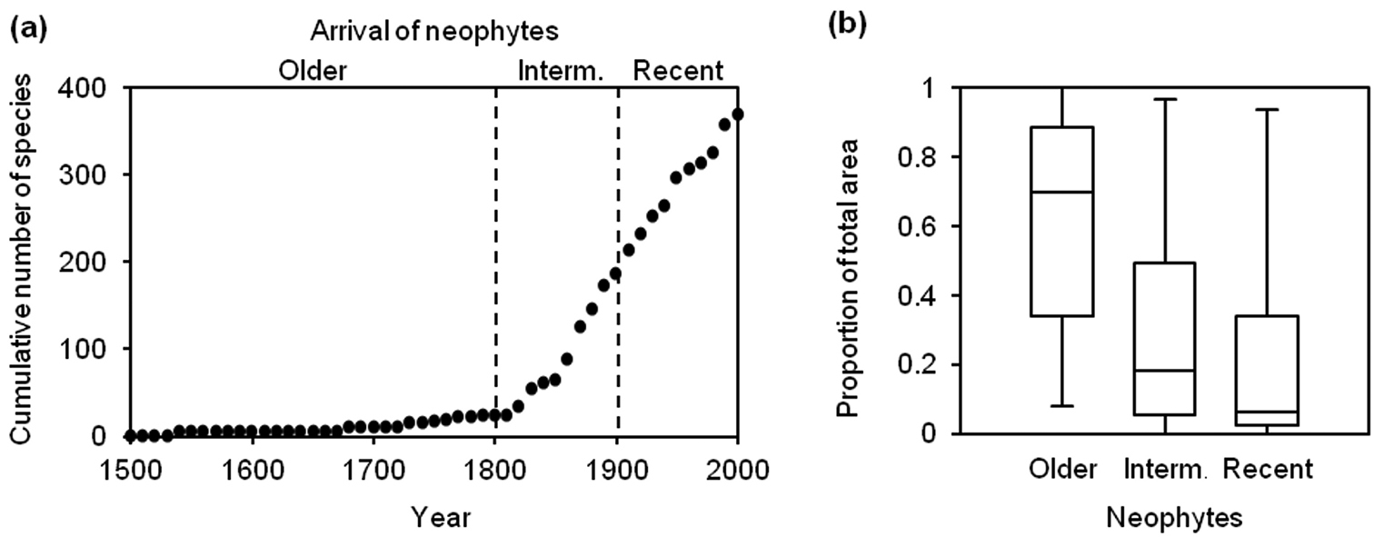
(a) Pattern of accumulation of neophyte species in the Friuli Venezia-Giulia region after the 15th century. Dashed lines divide the curve into three time periods used to differentiate three species groups: 1500–1800, a long period of gradual colonisation (older neophytes); 1800–1900, a first acceleration of the arrivals (intermediate neophytes); > 1900, a second acceleration (recent neophytes). (b) Box and whisker plots of the range sizes as a proportion of the total mapping units of three groups of neophytes differing in minimum residence time.

The dates of the first records in the study region were assembled from the checklist of Italian alien species (Celesti-Grapow et al. 2009) and from the major floristic works and published floristic papers for the Friuli Venezia Giulia region (Marchesetti 1896-97, Pospichal 1897-99, Gortani and Gortani 1905-06, Poldini 1980, Mezzena 1986, Poldini 1991, 2002, 2009). We observed a pattern of species accumulation over time (Fig. 1a). Following de Albuquerque et al. (2011b), neophytes were grouped according to three periods of arrival: (i) from 1500 until c. 1800, characterised by a slow increase in the number of alien species (23 species, about 6% of the total species number); (ii) from c. 1800 until c. 1900, characterised by an acceleration in the number of introductions (149 species, about 40% of the total species number); and (iii) from c. 1900 until the present, characterised by a further acceleration in the number of introductions (196 species, about 53% of the total species number). Hereafter, we refer to these groups as older neophytes (MRT = 200-500 years), intermediate neophytes (MRT = 100-200 years), and recent neophytes (MRT < 100 years).

Explanatory variables

We used the same grid to generate a series of explanatory variables quantifying climate, human-impact, and composition of the landscape. For each group we selected a first set of 35 variables of interest (Appendix S1).

For climatic variables, we considered annual precipitation (PREC) as an indicator of water availability and annual mean temperature (TEMP) as a measure of available energy. The data were retrieved from continuous raster-based climatic maps with a resolution of 100 × 100 m (1991–2008) provided by the Meteorological Observatory of Friuli Venezia Giulia (OSMER).

For variables of human-impact, we quantified population density for each cell (POP) using the dasymetric grid of population density disaggregated with Corine Land Cover and point survey data, as described in Gallego (2010), and obtained from the European Environment Agency (available at http://www.eea.europa.eu/ ). We measured the degree of urbanisation as the coverage of built-up areas (URB) (buildings, streets, and other artificial land uses) and as the total road length (ROAD) per cell. We also determined the proportion of agricultural land (AGR) as a further predictor of human disturbance. These land-cover variables were derived from the CORINE vector based map (2000), originally comprising 44 classes organized in three hierarchical levels (Servizio Sistema Informativo Territoriale e Cartografia - Direzione Centrale Pianificazione Territoriale, Autonomie Locali e Sicurezza, Trieste, Italy; available at http://www.regione.fvg.it/ ). These land-cover classes were obtained by merging the CORINE classes. To reduce collinearity, we only kept the ecologically most meaningful and least interrelated variables identified by calculating a Pearson’s correlation matrix for model fitting. Variables related to human-impact were strongly interrelated (r > 0.7), so we used only population density as a proxy of the overall level of human pressure and urban development (Appendix S2).

The composition of the landscape was described by the distribution of natural and semi-natural habitats in each cell, excluding agricultural and artificial habitats used as a proxy of human disturbance. Percentages of habitats were calculated from the CORINE biotopes map (1:50 000) of the study region (Servizio Valutazione Impatto Ambientale - Direzione Centrale Ambiente e Lavori Pubblici, Trieste, Italy; available at http://www.regione.fvg.it/ ). A standard classification of European habitats from the European Nature Information System (EUNIS; Davies et al., 2004, available at http://eunis.eea.europa.eu/habitats.jsp ) was chosen as a convenient platform for evaluating biological invasions in Europe (Vilà et al. 2007, Chytrý et al. 2008b, Pyšek et al. 2010). CORINE biotopes were transferred to the EUNIS habitat classification based on the classification links of Lapresa et al. (2004). We used a total of 29 habitat classes. The 29 landscape variables (i.e. the proportion of each class in the cells) was reduced to 2 using a principal components analysis (PCA), and keeping the first two orthogonal axes. The broken-stick method was used as stopping rule in the PCA. This method only retains the components associated with eigenvalues larger than the values given by the broken-stick distribution, providing an accurate estimate of the dimensionality of the data (Jackson 1993). PCA analyses retained two axes that explained 33% of the variation in the composition of the landscape (Appendix S3). The first axis (called ALP) had the highest loadings to alpine habitats constrained by environmentally stressful conditions; the second axis (called TERM) had the highest loadings with thermophilous habitats constrained by dry and warm conditions. We thus used a total of five variables (temperature, precipitation, population density, alpine habitats, and thermophilous habitats) for model fitting.

Data analysis

Statistical analyses were performed with all alien plants occurring in the study region and within separate groups of alien species defined by residence time. First, the relative roles of climatic, human, and landscape variables on the observed variation in species richness were assessed using ordinary least squares (OLS) regression. Given that we had no a priori hypotheses supporting interactions between the considered explanatory variables, we did not include any interaction terms in our model selection procedure. We performed a backward manual deletion procedure starting from the full model (P < 0.05). We standardised the response variables (i.e. species richness) to zero mean and unit standard deviation to make the parameter estimates comparable. To produce a set of non-negative standardised variables, a constant value of three was added to all values.

Second, we evaluated the robustness of the standardised regression coefficients of our non-spatial OLS models by comparing them with those of spatial models generated with spatial eigenvector mapping (SEVM) techniques (Borcard and Legendre 2002). Because autocorrelation usually causes further variables to become insignificant, but not insignificant variables to become significant, the backward-selected variables in OLS models were entered into the SEVM (Kühn 2007). The selection of the eigenvectors was implemented with a forward method that focused on minimising residual autocorrelation (Griffith and Peres-Neto 2006). A Gabriel connection was used to describe the spatial relationships between spatial units (Legendre and Legendre 1998). Gabriel networks approximate the rook scheme when the data are in a regular grid (as in our case). Using these short-distance connections is preferable (i.e. more conservative; Griffith 1996) to using inverse-decaying distances, since in most empirical data sets, residual spatial autocorrelation tends to be stronger at smaller distance classes (Bini et al. 2009). The spatial analyses were performed using Spatial Analysis in Macroecology (SAM) software (version 4.0; Rangel et al. 2010).

Third, we used hierarchical partitioning (HP) (Chevan and Sutherland 1991) to rank the importance of each variable most likely to affect variation in species richness. HP is an analytical method of multiple regression that quantifies the relative importance of each explanatory variable to the total explained variance of the regression model, both independently and together with the other explanatory variables, calculated for all possible candidate models. HP was conducted using the ‘hier.part’ package implemented in R version 2.14.1 (R Development Core Team 2011). The independent effects were tested using a randomization routine (n = 200), which gives Z-scores for the generated distribution of randomized independent contributions and a level of statistical significance (P) based on this score. We used a normal error distribution and R2 as a measure of goodness-of-fit. We then used the results of HP to compare the relative importance of each group of environmental variables (i.e. climate, human-impact, and landscape). Environmental sets were assembled using the percentages of independent effects derived by HP. The climatic set was assembled using the independent effects of temperature and precipitation, the human-impact set using the independent effect of population density, and the landscape set using the independent effects of alpine and thermophilous habitats.

Finally, we conducted partial regressions to partition the variation explained by environmental (backward-selected climatic, human-impact, and landscape variables) and spatial variables into independent and covarying components. The total explained variation in species richness was partitioned into three components (Borcard et al. 1992, Peres-Neto and Legendre 2010): (i) the non-spatial environmental variation (E), which is the fraction of the variation in species richness that can be explained by the environmental descriptors independently of any spatial structure; (ii) the spatial structuring in the species data that is shared by the environmental data (E∩S), i.e. induced spatial dependence, which is defined as the spatial structure of the response variables that exists due to the spatial structure of the explanatory variables; and (iii) the spatial patterns (S) in the species data that are not shared by the environmental data, due to large scale spatial trends and small scale autocorrelation generated by the species themselves (i.e. from biotic processes such as growth, dispersal, and mortality) or simply due to model misspecification (i.e. ignoring an important variable of spatial structure or falsely assuming a linear relationship that indeed is non-linear; Dormann et al. 2007, Anderson et al. 2010, Kühn and Dormann 2012). The variation explained in each model was reported as the adjusted R2 (R2adj), which takes the number of predictor variables and sample size into account to prevent the inflation of R2 values (Peres-Neto et al. 2006). When a negative R2adj was obtained, we interpreted it as a zero value (Peres-Neto et al. 2006), which means that not all fractions of one variation partitioning always add up to a perfect 100%. The partial regression analyses were implemented in the ‘vegan’ package for R.

Results

Range sizes decreased significantly from older to intermediate to recent neophytes (Fig. 1b, one-way ANOVA, F = 7.73, P < 0.001).

The multiple regression models showed several differences in the significance and rank of the standardised regression coefficients among separate groups of alien species defined by residence time (Table 1). For older neophytes, the model retained temperature and population density. For intermediate and recent neophytes, the models included temperature, population density, and thermophilous habitats. Temperature was the most important factor and was positively correlated with alien species richness in all the models. Positive partial coefficients were also found for the regression coefficients of the population density, but they were always substantially lower than those of temperature, especially for older neophytes. Thermophilous habitats had a weaker positive relationship with alien species in the models of intermediate and recent neophytes, suggesting that alien species richness is higher in dry and warm conditions.

Table 1.

Minimum adequate models for the relationships between alien species richness and the predictors (TEMP, annual mean temperature; POP, population density; TERM, thermophilous habitats) in the in the Friuli Venezia-Giulia region (Southern Alps) tested in the ordinary least squares (OLS) multiple regression models and in the spatial models generated with spatial eigenvector mapping (SEVM) techniques. The models are for (a) all neophyte plants occuring in the study region and within separate groups of neophytes defined by minimum residence time (MRT): (b) older neophytes (MRT = 200-500 yr), (c) intermediate neophytes (MRT = 100-200 yr), and (d) recent neophytes (MRT = <100 yr). Standardized regression coefficients (β) are presented.

  OLS       SEVM      
  β t P R2 β t P R2
(a) All neophytes       0.82       0.85
TEMP 0.558 7.895 <0.001 0.815 3.543 0.001
POP 0.444 6.293 <0.001 0.406 4.724 <0.001
TERM 0.209 3.610 <0.001 0.207 2.740 0.009
(b) Older neophytes 0.66 0.82
TEMP 0.685 7.033 <0.001 0.705 4.735 <0.001
POP 0.196 2.012 0.049 0.395 4.747 <0.001
(c) Intermediate neophytes 0.81 0.90
TEMP 0.557 7.710 <0.001 0.812 3.987 <0.001
POP 0.447 6.187 <0.001 0.319 4.329 <0.001
TERM 0.177 2.995 0.004 0.028 0.390 0.699
(d) Recent neophytes 0.72 0.84
TEMP 0.471 5.343 <0.001 0.246 1.478 0.147
POP 0.461 5.227 <0.001 0.356 4.347 0.001
TERM 0.237 3.283 0.002   0.137 1.828 0.075  

Including spatial filters in the model increased the amount of variance able to be explained, while the rank of the standardised regression coefficients of the variables was similar to OLS in all but the models for recent neophytes (Table 1). The effects of spatial filters on the P-values of the regression coefficients, however, were more important. Temperature was significant in the OLS model of recent neophytes but insignificant in the SEVM model and the thermophilous habitats in the models of intermediate and recent neophytes. Moreover, the standardised regression coefficients of predictors showed strong differences between the OLS and SEVM models. Temperature (e.g. for all and intermediate neophytes) and population density (e.g. for older neophytes) particularly had strong shifts in coefficients between the OLS and SEVM analyses (Table 1).

The results of hierarchical partitioning generally reflected those yielded by the regression models but produced slightly different results concerning the relative importance of some variables (Fig. 2a). The variable ranking indicated that both temperature and alpine habitats, followed by population density and precipitation, were the best predictors, with the highest independent effect on the number of alien species for older neophytes. For intermediate and recent neophytes, population density showed the largest independent effects followed by temperature. Considering the three sets of environmental variables (Fig. 2b), there was a reduction in the influence of climate and landscape, and an increase in the influence of human-impact, from the older neophytes to the recent neophytes (from 49% to 35% for climate, from 34% to 29% for landscape, and from 17% to 36% for human-impact).

Figure 2.

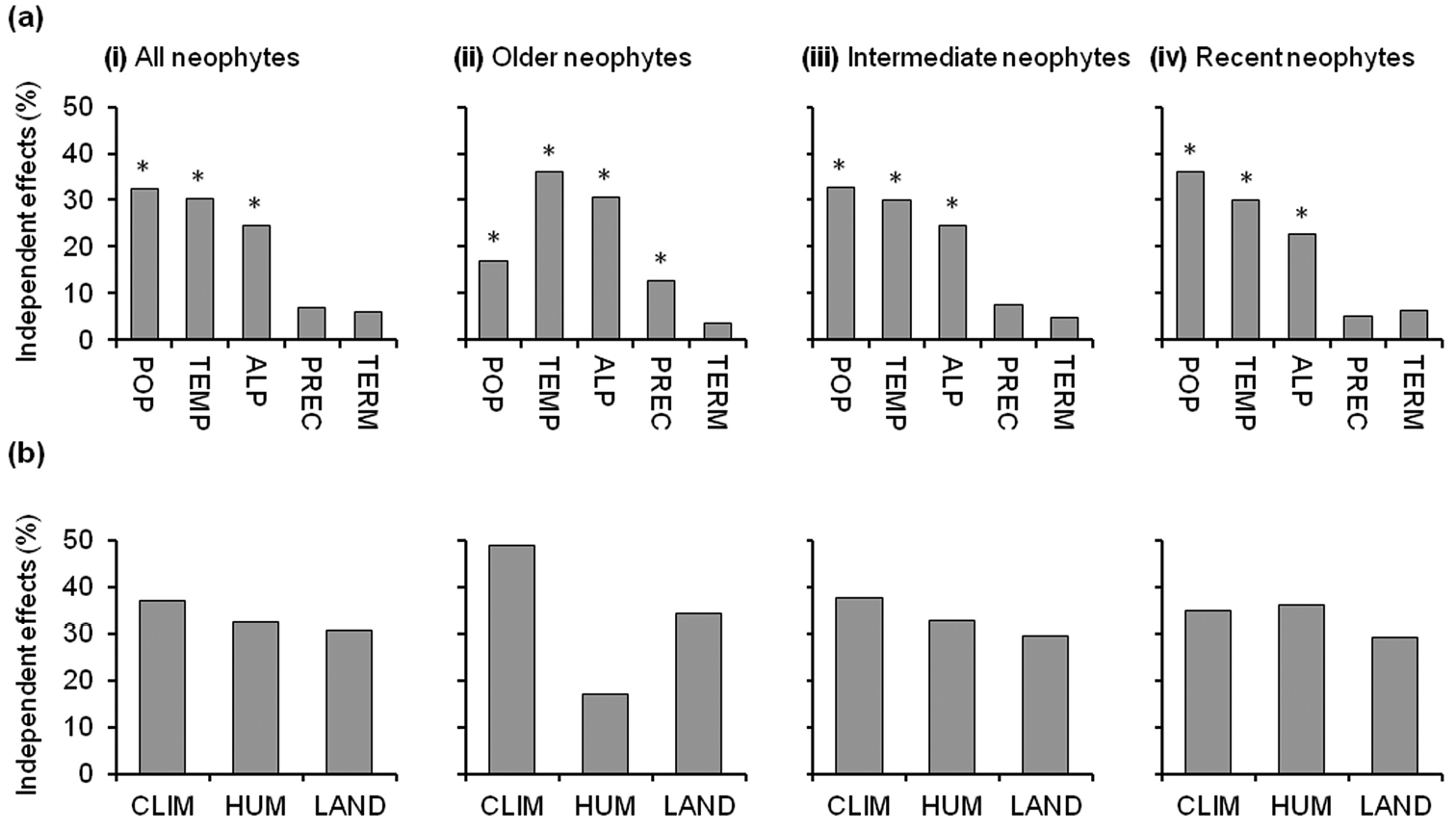
The relative independent effects of (a) environmental variables and (b) environmental variable sets (CLIM-climate, HUM-human-impact, and LAND-landscape) on species richness of (i) all neophytes, (ii) older neophytes, (iii) intermediate neophytes, and (iv) recent neophytes. Variables are ranked by the size of the independent effect in model (i) (i.e. all neophytes). Asterisks indicate statistical significance (P < 0.05) of the independent effect of each variable based on randomization tests (n = 200). POP, population density; TEMP, annual mean temperature; ALP, alpine habitats; PREC, annual precipitation; TERM, thermophilous habitats. Climate includes temperature and precipitation; human-impact includes population density; and landscape includes alpine and thermophilous habitats.

Partial regression analyses showed that most of the variation explained by the models is attributable to spatially structured environmental variation (E∩S, c.70-80%), while environment (E) and space (S) each had small independent effects (c.10-20%) (Fig. 3). The independent environmental effect (E), however, decreased and conversely the independent spatial effect (S) increased, from the older neophytes to the recent neophytes (from 14% to 9% for environment and from 11% to 18% for space).

Figure 3.

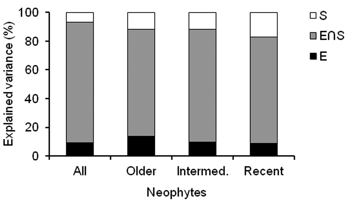
Variation partitioning of alien species richness per cell into environment and space for all neophytes, older neophytes, intermediate neophytes, and recent neophytes. The total variation explained was split into nonspatial environmental variation (E), spatially structured environmental variation (E∩S), and spatial structure not explained by the environmental variables (S). Results are expressed as part of the total explained variation for each component (i.e. values add up to 100%).

Discussion

The observed tendency for the sizes of the ranges of alien species to increase with minimum residence time in the Friuli Venezia Giulia region is consistent with patterns reported elsewhere in the world (Rejmánek 2000, Castro et al. 2005, Pyšek and Jarošík 2005, Ahern et al. 2010, de Albuquerque et al. 2011b). In general, the longer the time that a species is present in a region, the more it extends into its potential range because it has had more opportunities to be introduced several times at various locations and more time to disperse naturally, in order to overcome a ‘lag’ period (Kowarik 1995, Sakai et al. 2001, Gassó et al. 2012). Furthermore, residence time is also related to propagule pressure (Richardson and Pyšek 2006), i.e. alien species with longer residence times tend to produce and disperse more propagules.

This study also contributes to an understanding of how environmental-filtering (Weiher and Keddy 1999) and biotic processes, such as dispersal limitation (Svenning and Skov 2004), contribute to the distribution of alien species richness. We used environmental variables that summarise climatic conditions and human pressure to assess the role of environmental and disturbance filters for explaining patterns of alien species richness at a broader scale. Spatial patterns modelled by spatial eigenvector mapping were used to infer non-modelled processes acting at finer scales, such as dispersal and biotic interactions (Borcard et al. 2004) but also environmental factors that were not included in the analysis (Borcard et al. 2004, Dorman et al. 2007, Anderson et al. 2010).

Incorporating spatial filters in the models highlights several differences in the parameter estimates and shifts in coefficients between non-spatial and spatial regressions. These effects have also been observed in other studies (e.g. Dormann et al. 2007, Kühn 2007) and confirm the misestimation of the relationships between richness and its potential drivers when considering only non-spatial models. Why and when such shifts in coefficients between spatial and non-spatial methods occur, however, still remain largely unclear, and a recent study failed to support this or any other explanation for such shifts (Bini et al. 2009).

Role of environmental conditions

Environmental variables (E + E∩S) account for c. 80-90% of the explained variation in alien species richness, although 70–75% of this variation is spatially-structured (E∩S). The shared variation between explanatory variables and spatial descriptors is produced by induced spatial dependence (Peres-Neto and Legendre 2010), suggesting that environmental conditions are particularly important in determining alien species richness. As suggested by Cottenie (2005), including variables quantifying spatial structure should greatly improve the understanding of the factors that structure communities.

Specifically, we found strong differences in the importance of temperature and human disturbance on patterns of species richness in the three residence time groups. The association of alien species richness with temperature is stronger for groups with species having a longer residence time, which declines to become not significant for more recently arrived species, as shown in the spatial models. Furthermore, hierarchical partitioning shows a reduction in the influence of climate, from the older neophytes to the recent neophytes These results confirm the hypothesis that climate filtering (Weiher and Keddy 1999) has a key role in the post-introduction of alien species, because these species have had a longer time to adjust their distributions to the climatic conditions. The longer the residence time is, the greater the possibility for a species to have fully occupied its potential range in the study area (de Albuquerqueet al. 2011b, Gassó et al. 2012). Conversely, human pressure has a greater influence on species that arrived more recently, although its influence remains significant in all groups. This confirms that human pressures are key drivers of alien plant invasions. Anthropogenic changes to the landscape create niche opportunities for invaders, as pointed out in the ‘novel niche hypothesis’ (Shea and Chesson 2002). For example, abandoned fields and urban areas host a number of exotic species that cannot survive in adjacent forests (Lonsdale 1999). In addition, human pressure can shape the early stage of introduction, when humans determine the number of species introduced into a region and the number of attempts of introduction and/or number of individuals of each species introduced (‘propagule pressure hypothesis’; Lockwood et al. 2005).

Landscape variables instead show a trend similar to that observed for climate, with a reduction in the influence from the older neophytes to the recent neophytes. This trend could be due to the covariation among climatic and landscape variables. We particularly found a strong negative correlation between temperature and alpine habitats (r = -0.97; P < 0.001) and a meaningful negative correlation between precipitation and thermophilous habitats (r = -0.56; P < 0.001) (Appendix S2).

Role of spatial patterns

The shared variation between spatial descriptors and environmental variables is likely acting at broader spatial scales, accounting for environmental heterogeneity (e.g. climate and human pressures) and induced spatial dependence, whereas dispersal and biotic interactions such as competition, mortality, and social organisation are likely acting at finer spatial scales (Borcard et al. 2004, Cottenie 2005). We found an increasing fraction of the alien species richness explained solely by spatial descriptors (S) from the older neophytes (c.11%) to the recent neophytes (c.18%). This result suggests that fine-scale spatial patterns (those that can cause spatial autocorrelation), generated by dynamic processes regulating species richness, are important factors in determining alien plant invasions. Although these interpretations seem reasonable, recent discussions on the subject indicate that caution is required when attributing components of diversity to the outcome of these processes (Anderson et al. 2010, Smith and Lundholdm 2010, De Cáceres in press). The effect of environmental control and dispersal processes may be confounded by the frequent correlation between the spatial patterns created by dispersal limitation and the spatial arrangement of the environment (Smith and Lundholdm 2010, Anderson et al. 2010). Moreover, apparent spatial portions interpreted as ‘neutral’ could simply have been due to unmeasured environmental variables (Dormann et al. 2007, Anderson et al. 2010).

Conclusions

This study confirms the importance of considering residence time when studying spatial patterns of alien species richness and identifies residence time as a pivotal factor in the current distribution of alien species, i.e. climatic factors being most important for species with a longer residence time and factors related to human populations and habitat identity for species with shorter residence time. Our results also contribute to a better understanding of the influence of climate and human pressure on alien species richness and how these drivers shift their influences during the process of invasion. Additionally, the inclusion of spatial descriptors is important for explaining patterns of alien species and for unravelling the role of spatial autocorrelation generated by biotic processes.

Acknowledgements

We are grateful to Marisa Vidali for help in data collection and OSMER for providing climatic data. We thank William Blackhall for improving the English. We are grateful to two anonymous referees and the editor for the insightful comments that improved early drafts of the manuscript.

References
Ahern RG, Landis DA, Reznicek AA, Schemske DW (2010) Spread of exotic plants in the landscape: the role of time, growth habit, and history of invasiveness. Biological Invasions 12: 3157-3169. doi: 10.1007/s10530-010-9707-x
Anderson MJ, Crist TO, Chase JM, Vellend M, Inouye BD, Freestone AL, Sanders NJ, Cornell HV, Comita LS, Davies KF, Harrison SP, Kraft NJB, Stegen JC, Swenson NG (2010) Navigating the multiple meanings of β diversity: a roadmap for the practicing ecologist. Ecology Letters 14: 19-28. doi: 10.1111/j.1461-0248.2010.01552.x
Bini LM, Diniz JAF, Rangel T, Akre TSB, Albaladejo RG, Albuquerque FS, Aparicio A, Araújo MB, Baselga A, Beck J, Bellocq MI, Böhning-Gaese K, Borges PAV, Castro-Parga I, Chey VK, Chown SL, de Marco P, Dobkin DS, Ferrer-Castán D, Field R, Filloy J, Fleishman E, Gómez JF, Hortal J, Iverson JB, Kerr JT, Kissling WD, Kitching IJ, León-Cortés JL, Lobo JM, Montoya D, Morales-Castilla I, Moreno JC, Oberdorff T, Olalla-Tárraga MA, Pausas JG, Qian H, Rahbek C, Rodríguez MA, Rueda M, Ruggiero A, Sackmann P, Sanders NJ, Terribile LC, Vetaas OR, Hawkins BA (2009) Coefficient shifts in geographical ecology: an empirical evaluation of spatial and non-spatial regression. Ecography 32: 193-204. doi: 10.1111/j.1600-0587.2009.05717.x
Borcard D, Legendre P (2002) All-scale spatial analysis of ecological data by means of principal coordinates of neighbour matrices. Ecological Modelling 153: 51-68. doi: 10.1016/S0304-3800(01)00501-4
Borcard D, Legendre P, Avois-Jacquet C, Tuomisto H (2004) Dissecting the spatial structure of ecological data at multiple scales. Ecology 85: 1826-1832. doi: 10.1890/03-3111
Borcard D, Legendre P, Drapeau P (1992) Partialling out the Spatial Component of Ecological Variation. Ecology 73: 1045-1055. doi: 10.2307/1940179
Carboni M, Thuiller W, Izzi F, Acosta A (2010) Disentangling the relative effects of environmental versus human factors on the abundance of native and alien plant species in Mediterranean sandy shores. Diversity and Distributions 16: 537-546. doi: 10.1111/j.1472-4642.2010.00677.x
Castro SA, Figueroa JA, Muñoz-Schick M, Jaksic FM (2005) Minimum residence time, biogeographical origin, and life cycle as determinants of the geographical extent of naturalized plants in continental Chile. Diversity and Distributions 11: 183-191. doi: 10.1111/j.1366-9516.2005.00145.x
Celesti-Grapow L, Alessandrini A, Arrigoni PV, Banfi E, Bernardo L, Bovio M, Brundu G, Cagiotti MR, Camarda I, Carli E, Conti F, Fascetti S, Galasso G, Gubellini L, La Valva V, Lucchese F, Marchiori S, Mazzola P, Peccenini S, Poldini L, Pretto F, Prosser F, Siniscalco C, Villani MC, Viegi L, Wilhalm T, Blasi C (2009) Inventory of the non-native flora of Italy. Plant Biosystems 143: 386-430. doi: 10.1080/11263500902722824
Chevan A, Sutherland M (1991) Hierarchical partitioning. American Statistician 45: 90-96. doi: 10.2307/2684366
Chown SL, Hull B, Gaston KJ (2005) Human impacts, energy availability and invasion across Southern Ocean Islands. Global Ecology and Biogeography 14: 521-528. doi: 10.1111/j.1466-822x.2005.00173.x
Chytrý M, Jarošík V, Pyšek P, Hájek O, Knollová I, Tichý L, Danihelka J (2008a) Separating habitat invasibility by alien plants from the actual level of invasion. Ecology 89: 1541-1553. doi: 10.1890/07-0682.1
Chytrý M, Maskell LC, Pino J, Pyšek P, Vilà M, Font X, Smart SM (2008b) Habitat invasions by alien plants: a quantitative comparison among Mediterranean, subcontinental and oceanic regions of Europe. Journal of Applied Ecology 45: 448-458. doi: 10.1111/j.1365-2664.2007.01398.x
Chytrý M, Pyšek P, Wild J, Pino J, Maskell LC, Vilà M (2009) European map of alien plant invasions based on the quantitative assessment across habitats. Diversity and Distributions 15: 98-107. doi: 10.1111/j.1472-4642.2008.00515.x
Cottenie K (2005) Integrating environmental and spatial processes in ecological community dynamics. Ecology Letters 8: 1175-1182. doi: 10.1111/j.1461-0248.2005.00820.x
Davies CE, Moss D, Hill MO (2004) EUNIS habitat classification, revised 2004. European Environment Agency, Copenhagen and European Topic Centre on Nature Protection and Biodiversity (Paris).
de Albuquerque FS, Castro-Díez P, Rodríguez MA, Cayuela L (2011a) Assessing the influence of environmental and human factors on native and exotic species richness. Acta Oecologica-International Journal of Ecology 37: 51-57. doi: 10.1016/j.actao.2010.11.006
de Albuquerque FS, Castro-Díez P, Rueda M, Hawkins BA, Rodríguez MA (2011b) Relationships of climate, residence time, and biogeographical origin with the range sizes and species richness patterns of exotic plants in Great Britain. Plant Ecology 212: 1901-1911. doi: 10.1007/s11258-011-9962-7
De Cáceres M, Legendre P, Valencia R, Cao M, Chang LW, Chuyong G, Condit R, Hao Z, Hsieh CF, Hubbell S, Kenfack D, Ma K, Mi X, Supardi Noor N, Kassim AR, Ren H, Su SH, Sun IF, Thomas D, Ye W, He F (in press) The variation of tree beta diversity across a global network of forest plots. Global Ecology and Biogeography. doi: 10.1111/j.1466-8238.2012.00770.x
Dormann CF, McPherson JM, Araújo MB, Bivand R, Bolliger J, Carl G, Davies RG, Hirzel A, Jetz W, Kissling WD, Kühn I, Ohlemüller R, Peres-Neto PR, Reineking B, Schröder B, Schurr FM, Wilson R (2007) Methods to account for spatial autocorrelation in the analysis of species distributional data: a review. Ecography 30: 609-628. doi: 10.1111/j.2007.0906-7590.05171.x
Evans KL, Warren PH, Gaston KJ (2005) Does energy availability influence classical patterns of spatial variation in exotic species richness? Global Ecology and Biogeography 14: 57–65. doi: 10.1111/j.1466-822X.2004.00134.x
Gallego FJ (2010) A population density grid of the European Union. Population and Environment 31: 460-473. doi: 10.1007/s11111-010-0108-y
Gassó N, Thuiller W, Pino J, Vilà M (2012) Potential distribution range of invasive plant species in Spain. NeoBiota 12: 25-40. doi: 10.3897/neobiota.12.2341
Gortani L, Gortani M (1905-06) Flora friulana con speciale riguardo alla Carnia. Tipografia Gio. Batt. Doretti (Udine): (1) 1-225, (2) 1–519.
Griffith D (1996) Some guidelines for specifying the geographic weights matrix contained in spatial statistical models. In: Arlinghaus S (Eds). Practical handbook of spatial statistics. CRC Press (Boca Raton): 65-82.
Griffith DA, Peres-Neto PR (2006) Spatial modeling in ecology: The flexibility of eigenfunction spatial analyses. Ecology 87: 2603-2613. doi: 10.1890/0012-9658(2006)87[2603:SMIETF]2.0.CO;2
Hamilton MA, Murray BR, Cadotte MW, Hose GC, Baker AC, Harris CJ, Licari D (2005) Life-history correlates of plant invasiveness at regional and continental scales. Ecology Letters 8: 1066-1074. doi: 10.1111/j.1461-0248.2005.00809.x
Hodkinson DJ, Thompson K (1997) Plant dispersal: the role of man. Journal of Applied Ecology 34: 1484-1496. doi: 10.2307/2405264
Hubbell S (2001) The unified neutral theory of biodiversity and biogeography. Princeton University Press (Princeton).
Jackson DA (1993) Stopping Rules in Principal Components Analysis: A Comparison of Heuristical and Statistical Approaches. Ecology 74: 2204-2214. doi: 10.2307/1939574
Kowarik I (1995) Time lags in biological invasions with regard to the success and failure of invasive species. In: Pyšek P, Prach K, Rejmánek M, Wade M (Eds). Plant Invasions: General Aspects and Special Problems. SPB Academic Publishing (Amsterdam): 15-38.
Kowarik I (2003) Human agency in biological invasions: secondary releases foster naturalisation and population expansion of alien plant species. Biological Invasions 5: 293-312. doi: 10.1023/B:BINV.0000005574.15074.66
Kühn I (2007) Incorporating spatial autocorrelation may invert observed patterns. Diversity and Distributions 13: 66-69. doi: 10.1111/j.1472-4642.2006.00293.x
Kühn I, Dormann CF (2012) Less than eight (and a half) misconceptions of spatial analysis. Journal of Biogeography 39: 995-998. doi: 10.1111/j.1365-2699.2012.02707.x
Lapresa A, Angelici P, Festari I (2004) Gli habitat secondo la nomenclatura EUNIS: manuale di classificazione per la realtà italiana. APAT (Roma): 1–160.
Legendre P (1993) Spatial Autocorrelation: Trouble or New Paradigm? Ecology 74: 1659–1673. doi: 10.2307/1939924
Legendre P, Legendre L (1998) Numerical Ecology, 2nd edition. Elsevier Science (Amsterdam): xv + 853.
Lockwood JL, Cassey P, Blackburn T (2005) The role of propagule pressure in explaining species invasions. Trends in Ecology & Evolution 20: 223-228. doi: 10.1016/j.tree.2005.02.004
Lonsdale WM (1999) Global patterns of plant invasions and the concept of invasibility. Ecology 80: 1522-1536. doi: 10.1890/0012-9658(1999)080[1522:GPOPIA]2.0.CO;2
Marchesetti C (1896–97) Flora di Trieste e de’ suoi dintorni. Tipografia del LLoyd Austriaco (Trieste): 1–727.
Marini L, Gaston KJ, Prosser F, Hulme PE (2009) Contrasting response of native and alien plant species richness to environmental energy and human impact along alpine elevation gradients. Global Ecology and Biogeography 18: 652-661. doi: 10.1111/j.1466-8238.2009.00484.x
Mezzena R (1986) L’erbario di Carlo Zirnich (Ziri). Atti del Museo Civico di Storia Naturale di Trieste (Trieste): 1–519.
Peres-Neto PR, Legendre P (2010) Estimating and controlling for spatial structure in the study of ecological communities. Global Ecology and Biogeography 19: 174-184. doi: 10.1111/j.1466-8238.2009.00506.x
Peres-Neto PR, Legendre P, Dray S, Borcard D (2006) Variation partitioning of species data matrices: Estimation and comparison of fractions. Ecology 87: 2614-2625. doi: 10.1890/0012-9658(2006)87[2614:VPOSDM]2.0.CO;2
Poldini L (1980) Catalogo floristico del Friuli-Venezia Giulia e dei territori adiacenti. Studia Geobotanica 1: 313-474.
Poldini L (1991) Atlante corologico delle piante vascolari nel Friuli-Venezia Giulia. Inventario floristico regionale. Regione Autonoma Friuli-Venezia Giulia–Direzione Regionale Foreste e Parchi, Università degli Studi di Trieste-Dipartimento di Biologia (Udine): 1–900.
Poldini L (2002) Nuovo atlante corologico delle piante vascolari nel Friuli Venezia Giulia, Vol. Regione Autonoma Friuli-Venezia Giulia–Direzione Regionale Foreste e Parchi, Università degli Studi di Trieste–Dipartimento di Biologia (Udine): 1–529.
Poldini L (2009) Guide alla Flora – IV.  La diversità vegetale del Carso fra Trieste e Gorizia. Lo stato dell’ambiente. Ed. Goliardiche (Trieste): 1–732.
Pospichal E (1897-99) Flora des österreichischen Küstenlandes. Franz Deuticke (Leipzig und Wien): (1) 1–576, (2) 1–946.
Pyšek P, Bacher S, Chytrý M, Jarošík V, Wild J, Celesti-Grapow L, Gasso N, Kenis M, Lambdon PW, Nentwig W, Pergl J, Roques A, Sádlo J, Solarz W, Vilà M, Hulme PE (2010) Contrasting patterns in the invasions of European terrestrial and freshwater habitats by alien plants, insects and vertebrates. Global Ecology and Biogeography 19: 317-331. doi: 10.1111/j.1466-8238.2009.00514.x
Pyšek P, Jarošík V (2005) Residence time determines the distribution of alien plants. In: Inderjit S (Eds). Invasive plants: ecological and agricultural aspects. Birkhäuser Verlag (Basel): 77-96.
Pyšek P, Křivánek M, Jarošík V (2009) Planting intensity, residence time, and species traits determine invasion success of alien woody species. Ecology 90: 2734-2744. doi: 10.1890/08-0857.1
Pyšek P, Richardson DM, Rejmánek M, Webster GL, Williamson M, Kirschner J (2004) Alien plants in checklists and floras: towards better communication between taxonomists and ecologists. Taxon 53: 131-143. doi: 10.2307/4135498
R Development Core Team (2011) R: A language and environment for statistical computing. R Foundation for Statistical Computing, Vienna, Austria. http://www.R-project.org
Rangel TF, Diniz-Filho JAF, Bini LM (2010) SAM: a comprehensive application for Spatial Analysis in Macroecology. Ecography 33: 46-50. doi: 10.1111/j.1600-0587.2009.06299.x
Rejmánek M (2000) Invasive plants: approaches and predictions. Austral Ecology 25: 497-506. doi: 10.1046/j.1442-9993.2000.01080.x
Rejmánek M, Richardson DM, Pyšek P (2005) Plant invasions and invasibility of plant communities. In: Van der Maarel E (Eds). Vegetation ecology. Blackwell Science (Oxford): 332-355.
Richardson DM, Pyšek P (2006) Plant inva sions: merging the concepts of species invasiveness and community invasibility. Progress in Physical Geography 30: 409-431. doi: 10.1191/0309133306pp490pr
Sakai AK, Allendorf FW, Holt JS, Lodge DM, Molofsky J, With KA, Baughman S, Cabin RJ, Cohen JE, Ellstrand NC, McCauley DE, O’Neil P, Parker IM, Thompson JN, Weller SG (2001) The population biology of invasive species. Annual Review of Ecology and Systematics 32: 305-332. doi: 10.1146/annurev.ecolsys.32.081501.114037
Shea K, Chesson P (2002) Community ecology theory as a framework for biological invasions. Trends in Ecology & Evolution 17: 170-176. doi: 10.1016/S0169-5347(02)02495-3
Smith TW, Lundholm JT (2010) Variation partitioning as a tool to distinguish between niche and neutral processes. Ecography 33: 648-655. doi: 10.1111/j.1600-0587.2009.06105.x
Svenning JC, Skov F (2004) Limited filling of the potential range in European tree species. Ecology Letters 7: 565-573. doi: 10.1111/j.1461-0248.2004.00614.x
Vilà M, Pino J, Font X (2007) Regional assessment of plant invasions across different habitat types. Journal of Vegetation Science 18: 35-42. doi: 10.1658/1100-9233(2007)18[35:RAOPIA]2.0.CO;2
Wagner HH, Fortin MJ (2005) Spatial analysis of landscapes: Concepts and statistics. Ecology 86: 1975-1987. doi: 10.1890/04-0914
Weiher E, Keddy P (1999) Ecological assembly rules: perspectives, advances, retreats. Cambridge University Press (Cambridge): 1–430. doi: 10.1017/CBO9780511542237
Williamson M, Dehnen-Schmutz K, Kühn I, Hill M, Klotz S, Milbau A, Stout J, Pyšek P (2009) The distribution of range sizes of native and alien plants in four European countries and the effects of residence time. Diversity and Distributions 15: 158-166. doi: 10.1111/j.1472-4642.2008.00528.x
Wilson JRU, Richardson DM, Rouget M, Procheş Ş, Amis MA, Henderson L, Thuiller W (2007) Residence time and potential range: crucial considerations in modelling plant invasions. Diversity and Distributions 13: 11-22. doi: 10.1111/j.1472-4642.2006.00302.x
Appendix S1

List of all predictors considered.

Variable names and explanation Unit Mean ± SD Min Max
Climate
PREC Annual precipitation mm 1551 ± 365 976 2465
TEMP Annual mean temperature °C 10.18 ± 2.86 4.75 13.68
Human-impact
POP Population density per km2 126.5 ± 158.5 4.10 831.80
ROAD Road length km 99.37 ± 61.90 3.88 258.70
URB Total area covered by built-up elements % 7.30 ± 7.31 0.07 32.45
AGR Area covered by agricultural area % 34.54 ± 34.06 0.00 89.55
Land-use
A2 Littoral sediment % 1.73 ± 7.91 0.00 50.17
B1 Coastal dunes and sandy shores % 0.01 ± 0.08 0.00 0.57
C1 Surface standing waters % 0.13 ± 0.28 0.00 1.52
C2 Surface running waters % 0.25 ± 0.45 0.00 1.97
C3 Littoral zone of inland surface waterbodies % 1.65 ± 2.03 0.00 8.60
D2 Valley mires, poor fens and transition mires % 0.03 ± 0.11 0.00 0.53
D5 Sedge and reedbeds % 0.12 ± 0.61 0.00 4.26
E1 Dry grasslands % 2.20 ± 4.35 0.00 21.73
E2 Mesic grasslands % 1.60 ± 1.63 0.00 8.77
E3 Seasonally wet and wet grasslands % 0.01 ± 0.03 0.00 0.17
E4.3 Acid alpine and subalpine grassland % 0.64 ± 1.74 0.00 10.36
E4.4 Calcareous alpine and subalpine grassland % 1.81 ± 2.68 0.00 10.14
E4.5 Alpine and subalpine enriched grassland % 0.15 ± 0.42 0.00 1.86
F2 Arctic, alpine and subalpine scrub % 4.47 ± 7.15 0.00 31.88
F3 Temperate and mediterranean-montane scrub % 1.75 ± 3.49 0.01 21.39
F9 Riverine and fen scrubs % 0.12 ± 0.27 0.00 1.47
G1.1 Riparian and gallery woodland % 0.67 ± 0.97 0.00 3.37
G1.3 Mediterranean riparian woodland % 0.00 ± 0.01 0.00 0.10
G1.4 Broadleaved swamp woodland not on acid peat % 0.08 ± 0.22 0.00 1.05
G1.6 [Fagus] woodland % 13.69 ± 16.63 0.00 55.24
G1.7 Thermophilous deciduous woodland % 6.53 ± 9.51 0.00 46.33
G1.8 Acidophilous [Quercus]-dominated woodland % 2.31 ± 5.66 0.00 27.32
G1.A Meso- and eutrophic [Quercus] and related woodland % 1.78 ± 4.00 0.00 20.71
G3.1 [Abies] and [Picea] woodland % 7.59 ± 15.17 0.00 55.17
G3.2 Alpine [Larix] - [Pinus cembra] woodland % 1.42 ± 2.33 0.00 8.57
G3.5 [Pinus nigra] woodland % 3.88 ± 6.47 0.00 23.82
H2 Screes % 0.75 ± 1.31 0.00 6.84
H3 Inland cliffs, rock pavements and outcrops % 1.37 ± 2.42 0.00 9.97
  H4 Snow or ice-dominated habitats % 0.02 ± 0.15 0.00 1.13
Appendix S2

Pearson correlations between explanatory variables (TEMP, annual mean temperature; PREC, annual precipitation; POP, population density; ROAD, road length; URB, total area covered by built-up elements; AGR, area covered by agricultural area; ALP, alpine habitats; TERM, thermophilous habitats).

  TEMP PREC POP ROAD URB AGR ALP
PREC -0.563            
POP 0.574 -0.412
ROAD 0.721 -0.325 0.744
URB 0.711 -0.505 0.916 0.827
AGR 0.843 -0.699 0.498 0.651 0.724
ALP -0.971 0.482 -0.512 -0.654 -0.631 -0.754
TERM 0.045 -0.556 0.004 -0.079 0.088 0.306 0.000
Appendix S3

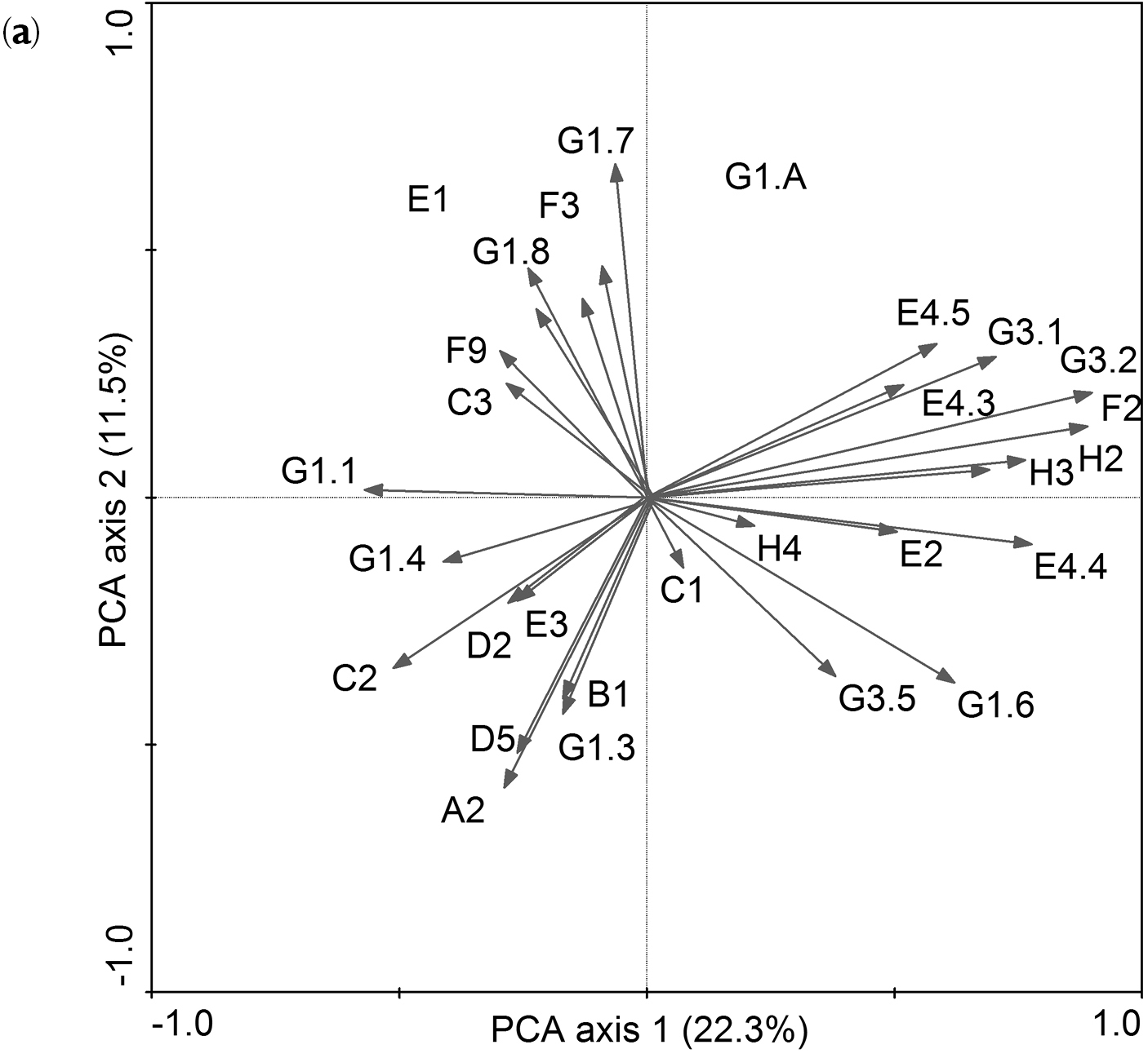
(a) Principal components analysis (PCA) diagram of 29 habitat classes, for codes of habitat classes please see Appendix S1

(b) Eigenvector scores of 29 habitat classes in two main PCA axes. Values are ranked in order of absolute magnitude along PCA 1. The five highest absolute eigenvector scores for each PCA axis are indicated in bold. Values in parentheses indicate variance accounted for by each axis.

Habitat PCA1 - ALP
(22.3%)
PCA2 - TERM
(11.5%)
G3.2 Alpine [Larix] - [Pinus cembra] woodland 0.899 -0.211
F2 Arctic, alpine and subalpine scrub 0.890 -0.143
E4.4 Calcareous alpine and subalpine grassland 0.777 0.094
H2 Screes 0.764 -0.075
G3.1 [Abies] and [Picea] woodland 0.704 -0.284
H3 Inland cliffs, rock pavements and outcrops 0.691 -0.056
G1.6 [Fagus] woodland 0.621 0.374
E4.5 Alpine and subalpine enriched grassland 0.585 -0.311
G1.1 Riparian and gallery woodland -0.570 -0.015
E4.3 Acid alpine and subalpine grassland 0.518 -0.227
E2 Mesic grasslands 0.505 0.070
C2 Surface running waters -0.492 -0.349
G3.5 [Pinus nigra] woodland 0.381 0.361
G1.4 Broadleaved swamp woodland not on acid peat -0.322 -0.095
A2 Littoral sediment -0.282 -0.644
E3 Seasonally wet and wet grasslands -0.268 -0.200
D5 Sedge and reedbeds -0.262 -0.600
E1 Dry grasslands -0.260 0.494
D2 Valley mires, poor fens and transition mires -0.249 -0.188
F9 Riverine and fen scrubs -0.238 0.246
H4 Snow or ice-dominated habitats 0.217 0.058
C3 Littoral zone of inland surface waterbodies -0.195 0.187
B1 Coastal dunes and sandy shores -0.189 -0.462
G1.A Meso- and eutrophic [Quercus] and related woodland -0.187 0.330
G1.3 Mediterranean riparian woodland -0.182 -0.464
G1.8 Acidophilous [Quercus]-dominated woodland -0.138 0.421
F3 Temperate and mediterranean-montane scrub -0.085 0.484
C1 Surface standing waters 0.073 0.142
G1.7 Thermophilous deciduous woodland -0.040 0.672