


(C) 2013 Denys Yemshanov. This is an open access article distributed under the terms of the Creative Commons Attribution License 3.0 (CC-BY), which permits unrestricted use, distribution, and reproduction in any medium, provided the original author and source are credited.
For reference, use of the paginated PDF or printed version of this article is recommended.
Citation: Yemshanov D, Frank FH, Ducey MJ, Haack RA, Siltanen M, Wilson K (2013) Quantifying uncertainty in pest risk maps and assessments: adopting a risk-averse decision maker’s perspective. In: Kriticos DJ, Venette RC (Eds) Advancing risk assessment models to address climate change, economics and uncertainty. NeoBiota 18: 193–218. doi: 10.3897/neobiota.18.4002
Pest risk maps are important decision support tools when devising strategies to minimize introductions of invasive organisms and mitigate their impacts. When possible management responses to an invader include costly or socially sensitive activities, decision-makers tend to follow a more certain (i.e., risk-averse) course of action. We presented a new mapping technique that assesses pest invasion risk from the perspective of a risk-averse decision maker.
We demonstrated the approach by evaluating the likelihood that an invasive forest pest will be transported to one of the U.S. states or Canadian provinces in infested firewood by visitors to U.S. federal campgrounds. We tested the impact of the risk aversion assumption using distributions of plausible pest arrival scenarios generated with a geographically explicit model developed from data documenting camper travel across the study area. Next, we prioritized regions of high and low pest arrival risk via application of two stochastic ordering techniques that employed, respectively, first- and second-degree stochastic dominance rules, the latter of which incorporated the notion of risk aversion. We then identified regions in the study area where the pest risk value changed considerably after incorporating risk aversion.
While both methods identified similar areas of highest and lowest risk, they differed in how they demarcated moderate-risk areas. In general, the second-order stochastic dominance method assigned lower risk rankings to moderate-risk areas. Overall, this new approach offers a better strategy to deal with the uncertainty typically associated with risk assessments and provides a tractable way to incorporate decision-making preferences into final risk estimates, and thus helps to better align these estimates with particular decision-making scenarios about a pest organism of concern. Incorporation of risk aversion also helps prioritize the set of locations to target for inspections and outreach activities, which can be costly. Our results are especially important and useful given the huge number of camping trips that occur each year in the United States and Canada.
Risk aversion, stochastic dominance, decision-making under uncertainty, pest risk mapping, firewood movement, pathway invasion model
Management of invasive species populations often requires making decisions about allocating scarce resources for surveillance or eradication of newly detected incursions. To aid in the decision-making process, agencies responsible for monitoring and controlling invasive species, such as the USDA Animal and Plant Health Inspection Service (APHIS) in the U.S. (
In cases where the need to manage invasive pest populations prompts calls for irreversible, costly or socially sensitive actions, decision-makers tend to follow a more certain course of action, thus exhibiting risk-averse behavior (
When decision-makers follow a risk-averse strategy, the presence of uncertainty in pest risk assessments inevitably changes decision outcomes about managing the pests. However, uncertainty has rarely been represented in assessments of new pest incursions in a geographical domain. At best, pest risk maps presented uncertainty as separate maps or a combination of coarse risk-uncertainty classes (
In this paper, we present a new risk mapping technique that helps quantify uncertainty in pest risk assessments from the perspective of a risk-averse decision maker. We consider a particular case of risk mapping when a decision-maker faces the problem of prioritizing a set of locations in a geographical domain based on imprecise estimates of the likelihood of pest arrival in a given area. Our goal with this paper is to present the approach of prioritizing uncertain outcomes of ecological invasions that would agree with a risk-averse decision-making strategy, and also to explore how the notion of risk-aversion changes the delineation of pest risk in a geographical domain.
In general, humans tend to place relatively low weights on uncertain outcomes and relatively high weights on certain outcomes (
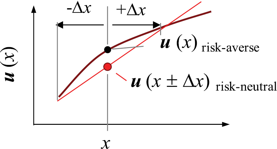
The expected utility function (EUF) concept. The EUF value can be interpreted as analogous to a decision-making priority that indicates the degree of importance for the decision-maker of a particular geographical site that is under risk of infestation. Bold line depicts an example of a concave EUF that denotes risk-averse decision-making preferences. The concavity condition means that a more certain amount of valuables (or degree of importance for the decision-maker) (u(x)) would always be preferred over a less certain choice (u(x ± Δx) with the same expected value, x. Dashed line shows an example EUF for a risk-neutral decision-maker (i.e., one who is indifferent between more certain and less certain choices with the same expected value).
The notion of risk-averse decision preferences can be embedded into the process of mapping risks of pest invasions. In our case, the concept of payoff can be thought as analogous to estimating anticipated losses from an invasive organism (or the likelihood of an organism’s arrival). Conceptually, the EUF value (Fig. 1) can be interpreted as analogous to a decision-making priority that indicates the degree of importance for the decision-maker of a particular geographical site that is under risk of infestation. Clearly, any rational decision-maker would assign a higher priority to geographical locations with a higher and more certain likelihood (or anticipated impact) of invasion. By adding the notion of risk-aversion we imply that the assessment of pest invasion risk should be done from the point of view of a decision-maker whose EUF is concave. In short, the notion of risk-aversion means that pest risk assessments (which, in our case as well as in general, translate to prioritization schemes) should include some sort of penalty for uncertain choices.
The use of the EUF’s concavity assumption for representing risk-averse behavior offers a formal treatment of risk aversion without the need to explicitly define the shape of the utility function. Essentially, the concavity condition is a very basic definition of general risk-averse preferences (i.e., by eliminating the cases when the decision-maker is risk-neutral or risk-seeking) and does not define a specific range of risk-averse preferences (such as moderate to extreme risk aversion). While it is possible to impose further restrictive assumptions on the type of risk-averse behavior – for instance, by assuming a particular functional form of the EUF or limiting the degree of risk aversion to an upper and lower bounds (
We consider a pest risk map that prioritizes geographical locations across a landscape based on the likelihood that the pest will arrive at a previously non-invaded locale. Ultimately, the assignment of decision-making priorities to a particular geographical location may depend on the decision-maker’s perception of uncertainty in the assessment of the impact of the pest invasion. In this paper, we explore how the incorporation of risk-averse decision preferences changes the prioritization of areas of high and low pest invasion risk in a geographical setting. We use distributions of plausible invasion scenarios generated by a stochastic model to predict the movement of an invasive organism across a heterogeneous landscape. We then delineate regions of high and low risk of pest arrival across the landscape via the application of two simple stochastic ordering techniques, one of which incorporates the notion of risk aversion. For consistency, we use ordering techniques from the same family based on the stochastic dominance (SD) rule. Finally, we identify geographical regions in a landscape where adding the notion of risk aversion changes the location’s pest risk value considerably.
The stochastic dominance rule is a form of stochastic ordering that compares a pair of distributions. The concept was previously applied to compare distributions of investment portfolio returns in financial valuation studies (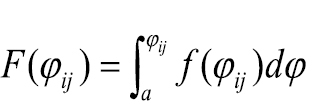 and
and 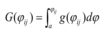 . Location f dominates g by the first-degree stochastic dominance rule (FSD) if
G(φij) – F(φij) ≥ 0 for all φij, and G(φij) – F(φij) > 0 for at least one φij. (1)
The FSD rule implies that the CDFs of f and g do not cross each other (Fig. 2A). The test for FSD also supposes that a decision-maker will always prefer the “higher-value” outcome (
The FSD conditions may fail when differences between G(φij) and F(φij) are small. Alternatively, second-degree stochastic dominance (SSD) provides weaker but more selective discrimination by comparing the integrals of the CDFs for F(φij) and G(φij): 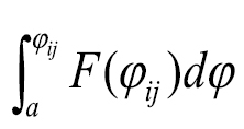 and
and 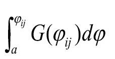 . Location f dominates the alternative g by SSD if
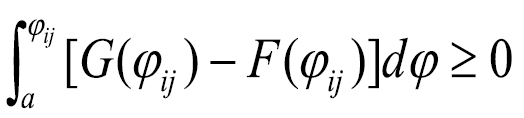 for all φij, and
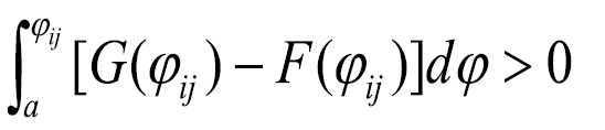 for at least one φij. (2)
The SSD rule implies that the integrals of the CDFs for F(φij) and G(φij) do not cross (Fig. 2B). The SSD condition adds the assumption that the decision-maker is risk-averse, that is the dominance relationships based on the SSD rule (Eq. 2) satisfy the assumption that the decision-maker’s EUF is concave (
The SSD and FSD tests are pairwise comparisons. However, our study required evaluating a set of N multiple geographical locations, or map elements, that constituted a landscape. For each rule, we applied multiple pairwise stochastic dominance tests of map elements to delineate a subset of elements, À1, from the total set N such that each element of À1 could not be dominated by any element in the rest of the set, N - À1. Formally, a non-dominant subset À1 is equivalent to an “efficient set” in financial investment valuation literature (
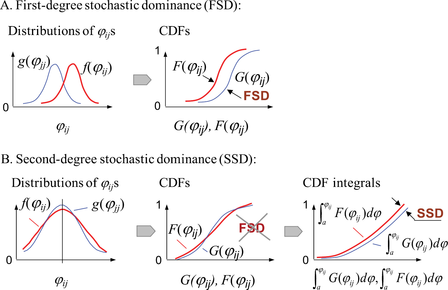
First-degree and second-degree stochastic dominance rules: A distributions, f(φij) and g(φij), of camper travel probabilities (φij) at two corresponding map locations, f and g B the cumulative distribution functions (CDFs), F(φij) and G(φij), of f(φij) and g(φij) in Fig. 1 (a). “FSD” indicates the first-degree stochastic dominance conditions are satisfied (i.e., G(φij) and F(φij) do not cross each other) C two additional example distributions of pest arrival rates at f and g D in this case, CDFs of f(φij) and g(φij) cross each other so that the first-degree stochastic dominance conditions fail E the integrals, 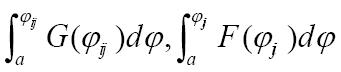 , of the CDFs. “SSD” indicates the second-degree stochastic dominance conditions are met (i.e.,
 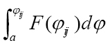 and
and 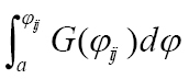 do not cross each other).
The stochastic dominance rule assumes a very broad range of decision-making behaviors and has relatively low ability to discriminate small non-dominant sets. To improve the discriminative capacity, some alternative metrics have been proposed. The stochastic dominance with respect to a function, or SDRF (
We explored the impact of decision-maker risk-aversion with a North American case study that estimates the likelihood of wood-boring forest pests arriving in firewood at campgrounds on U.S. federal lands in the 49 U.S. states by travelers from the continental U.S. and Canada. The potential for accidental, long-distance transport of alien species with recreational travel has become a topic of considerable concern in North America (
While the problem of moving forest pests with firewood is well recognized (
We used the NRRS data set to undertake spatial stochastic pathway simulations of potential movements of invasive pests with firewood carried by campers. Spatial stochastic models have been increasingly used for assessing risks of ecological invasions (
Our choice of a network-based model was aimed at emphasizing the importance of human-assisted movement of invasive organisms over long distances, a phenomenon that many classical dispersal models cannot predict well (see
We used the NRRS dataset to build a matrix of n × n origin–destination locations, where each matrix element defined the number of visits for a particular pair of origin–destination locations (i.e., the total number of reservations between a particular origin ZIP code and destination campground). Because the original NRRS records encompassed more than 500 000 unique spatial locations, we aggregated the data to a grid of 15x15 km cells. This aggregation decreased the size of the matrix and reduced the computational burden. The NRRS data were then parsed into a set of unique pathway segments, each connecting an origin map cell, i, and a destination map cell, j, in the network. Subsequently, the cumulative number of visits (based on the NRRS reservations) for each pathway segment ij were used to build an n × n pathway matrix where each element defined the rate, pij, of camper movement (and by extension, firewood-facilitated pest transport) from cell i to cell j. The pathway matrix stored the pij values for all possible pairs of (i, j) cells in the transportation network:
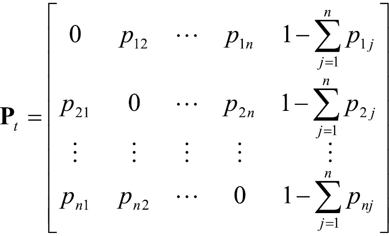 (3)
(3)
where the elements  describe the probability that camper travel between i and j did not occur and
pij = mijλ (4)
where mij is the total number of reservations for the origin-destination vector ij and λ is a scaling parameter.
Ideally, the scaling parameter λ would define the likelihood that a pest is moved with firewood from any location i to j. In fact, knowing the precise value of λ would be critical in order to estimate pij exactly. However, our study did not require precise estimates of λ because we had the more basic aim of prioritizing the geographical locations (i.e., map cells) according to their level of risk. In short, our goal was to order the full set of map cells in the dimension of high–low relative infestation risk via multiple pairwise tests for first- and second-degree stochastic dominance (as described in Eqs. 1 and 2). In this case, the value of λ needed only to besufficiently small to ensure that the sum of transmission rate values in the Pt matrix rows was below 1:
 . (5)
. (5)
We then used the Pt matrix to generate stochastic realizations of potential movements of campers (and by extension, pest-infested firewood) from a given cell i to other cells with recreational travel. With i set as the point of “origin”, the model simulated subsequent camper movements from i to other destination cells j by extracting the transmission probabilities from Pt associated with i (Fig. 3). The process continued until a selected destination node had no outgoing paths or a terminal state was chosen based on the elements  in Pt. Finally, for each pair of origin–destination locations (i, j), a transmission probability, φij, was estimated from the number of times the camper arrived at j from i over K multiple stochastic model realizations
φij = Jij / K (6)
where Jij is the number of individual pathway simulations where a camper originated at i and ultimately arrived at j, and K is the total number of individual simulations of pathway spread from i (for this study, K = 2×10⁶ for each i). The values of φij were estimated for each (i, j) pair of origin–destination cells, requiring a total of K×[n (n-1)] pathway simulations.
We used the transmission probabilities φij (which, in relative terms, depict the potential of invasive pests to be moved by recreational travelers) to order the map cells across Canada and the U.S. in dimensions of high-low risk. We built separate maps for each of the continental 49 U.S. states and nine Canadian provinces (including the Yukon Territory). For each potential origin map cell, the model generated a list of other cells (with corresponding transmission probabilities φij) to which the movement of campers (and, in turn, forest pests carried by firewood) was most likely. Since our primary focus was to estimate the risk of pest movement to a particular state or province, we rearranged the results so each cell i outside of a state (province) of interest, k, had an associated distribution of thetransmission probabilities φij (j ∈ k), from that location to the state of interest (Fig. 3). In short, this distribution described the degree of the location’s invasivenessin relation to the state (province) of interest.
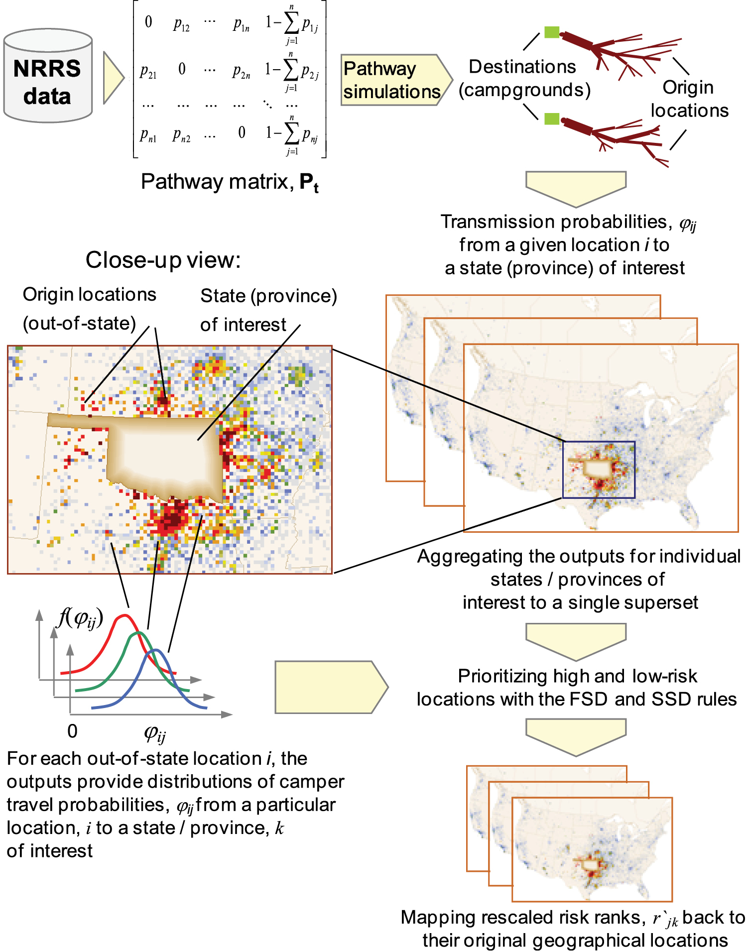
Mapping risks that invasive pests may be carried with infested firewood by campers (the analysis summary).
Assuming that the map for each state (province) of interest k had nk external locations that could potentially serve as sources of future pest arrivals with camper travel, the analysis produced a total (i.e., across all k) of N =  distributions of the jij transmission probability values. We then applied the FSD and SSD rules to this superset of distributions so that we could order them in the dimension of highest-to-lowest risk of transmission from i to k. Thus, each cell i was given two partial risk ranks, rik SSD and rik FSD, of pest movement from i to k by campers. Importantly, since partial ordering of the distributions of transmission probabilities was done in a single superset (that included all sets of outputs representing risks of movement to all k states / provinces of interest), the final risk ranks for different states and provinces can be compared one with another.
Our next goal was to compare the ranks generated with the FSD and SSD techniques and to explore how much the risk aversion assumption in the delineations based on the SSD rule changed the geographical patterns of risk across the study area. Because the SSD rule is weaker than FSD and usually produces smaller-size non-dominant sets (
Figure 4 depicts example maps of the rescaled risk ranks for Texas and California generated, using the second-degree stochastic dominance rule. (The maps of risk rankings based respectively, on the first- and second-degree stochastic dominance rules for the other U.S. states and the Canadian provinces are shown in online Appendices 1 and 2). The maps suggest some basic geographic trends in campers’ travel behavior. First, the highest-risk out-of-state locations (i.e., from where the movement of infested firewood is the most likely) are usually in close proximity to the state (provincial) border or, at longer travel distances, are associated with major urban centers. In addition, prominent recreational destinations such as Grand Canyon National Park (AZ) or Zion National Park (UT) are also high-risk locations. Notably, there are distinctive regional trends in camper behavior. For instance, interior states in the mid-western and southeastern U.S. are characterized by predominantly local and medium-range travel from surrounding areas. While states in these regions have few high-profile recreational destinations such as national parks, they have a dense and fairly uniform network of campgrounds, situated near major water bodies or public forest lands, which are used more often by casual or short-term campers.
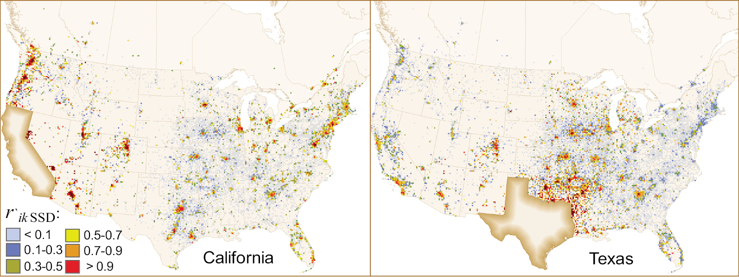
Examples of risk maps depicting the potential of invasive forest pests to be moved by recreational travelers to the states of Texas and California. The risk rank values are based on the second-degree stochastic dominance rule (SSD), which incorporates risk-averse decision preferences. The maps for the other U.S. states, Canadian provinces and the Yukon Territory can be found in online Appendix 2.
The western U.S. has vast areas of sparsely populated land, and so has a higher relative proportion of long-distance sources of campers (and thus potential firewood-associated pests) than the eastern U.S. The risk of pests being moved by campers returning to Canada is relatively low. However, the largest Canadian cities, such as Toronto (ON), Montreal (QC) and Vancouver (BC), have relatively high risks of being potential sources of infestations in neighboring U.S. states.
We investigated the geographic differences between the risk rank maps based on the FSD and SSD criteria. Figure 5 and online Appendix 3 present maps of differences in rank values, Δr`ik = r`ik FSD – r`ij SSD, composed for individual states and provinces. Overall, the FSD and SSD approaches provided similar delineations of the locations ranked with the most extreme risks, i.e., above 0.95 or below 0.05 (Table 1). The greatest differences between the ranks based on the FSD and SSD criteria were found in the areas in the peri-urban and rural zones (since information about camper travel to these locations is expected to be less certain because of a lack of well-documented links from the NRRS data).
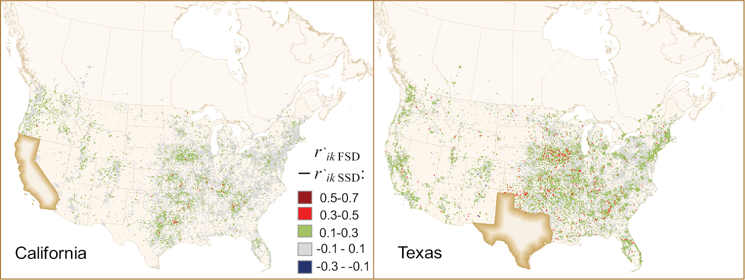
Maps of rank differences, Δr`ik = r`ik FSD – r`ik SSD, between the delineations based on first- and second-degree stochastic dominance for Texas and California. Positive values indicate that the SSD-based risk rank is lower than the FSD-based rank (so adding the notion of risk aversion decreases the risk rank). The maps for the other U.S. states, Canadian provinces and the Yukon Territory can be found in online Appendix 3.
For moderate risk ranks between 0.05 and 0.95, the methods appeared to place differing levels of emphasis on certainty in the φij transmission probabilities. The SSD approach seemed to decrease the risk rank’s value when the variation of the probability (i.e. uncertainty) was high and generally assigned lower rank values than the approach based on the FSD rule. This tendency is particularly evident in the range of moderate ranks 0.05–0.5 (Table 1). For example, almost 90% of ranks assigned to a 0.25–0.5 range in the FSD classification were classified into the 0.05–0.25 range in the SSD classification. Similarly, 72% of low-risk ranks classified within the range of 0.05–0.25 in the FSD classification had an SSD rank below 0.05, and roughly 83% of locations with FSD ranks in the 0.5–0.75 range were assigned lower risk ranking in the SSD delineations (Table 1).
Correspondence between the FSD and SSD rank classes as a percent of the map area. The numbers in the diagonal show the percentages of the map area where the rank class was the same in both FSD and SSD rankings. The largest percentage values in each row are marked on bold.
| Risk rank based on the FSD rule | Risk rank based on the SSD rule | |||||
|---|---|---|---|---|---|---|
| 0–0.05 (lowest) | 0.05–0.25 | 0.25–0.5 | 0.5-0.75 | 0.75–0.95 | 0.95–1 (highest) | |
| 0–0.05 (lowest) | 100 | |||||
| 0.05–0.25 | 72.2 | 27.7 | 0.1 | |||
| 0.25–0.5 | 0.7 | 89.8 | 7.7 | 1.8 | ||
| 0.5–0.75 | 30.5 | 52.8 | 15.0 | 1.7 | ||
| 0.75–0.95 | <0.01 | 3.5 | 24.6 | 71.0 | 0.9 | |
| 0.95–1 (highest) | 2.6 | 97.4 | ||||
Online Appendix 4 presents summaries of the differences, for individual states and provinces, between the FSD and SSD ranks allocated to broad rank classes: 0–0.05, 0.05–0.25, 0.5–0.75, 0.75–0.95 and 0.95–1. Most of the changes in rank values occurred in low–medium rank classes between 0.05 and 0.5, which is consistent with Table 1. For many states and provinces, the difference between the FSD and SSD-based ranks was at least one rank class (e.g., ranks in a 0.25–0.5 range under the FSD rule were assigned to a 0.05–0.25 range under the SSD rule).
The maps in online Appendix 3 suggest that geographical patterns of changes between the FSD and SSD rank values, Δr`ik, can be grouped into three general types. The first type represents states with very high volumes of out-of-state recreational visits (and thus higher risks of pest arrival with infested firewood from elsewhere), such as California and Texas (Table 2, Appendix 3). For these states, the high Δr`ik values are uniformly distributed in rural and suburban regions across much of the entire central and western U.S. However, the difference between the FSD and SSD ranks in large urban areas appeared to be small (Fig. 5).
State and provincial summaries based on the mean rank values, r`ik FSD and r`ik FSD.
| Country | State / Province | FSD-based risk rank | SSD-based risk rank | ||
|---|---|---|---|---|---|
| Mean r`ik FSD | Relative rank | Mean r`ik SSD | Relative rank | ||
| US | Texas | 0.283 | 1 | 0.202 | 1 |
| US | Arkansas | 0.251 | 2 | 0.184 | 3 |
| US | California | 0.246 | 4 | 0.202 | 2 |
| US | Missouri | 0.246 | 3 | 0.167 | 4 |
| US | Tennessee | 0.226 | 5 | 0.157 | 5 |
| US | Colorado | 0.215 | 6 | 0.140 | 7 |
| US | Georgia | 0.201 | 8 | 0.143 | 6 |
| US | Florida | 0.205 | 7 | 0.128 | 8 |
| US | Illinois | 0.197 | 9 | 0.121 | 10 |
| US | Iowa | 0.185 | 10 | 0.123 | 9 |
| US | Oklahoma | 0.179 | 11 | 0.117 | 11 |
| US | Washington | 0.169 | 12 | 0.109 | 15 |
| US | Oregon | 0.168 | 13 | 0.110 | 14 |
| US | Arizona | 0.161 | 15 | 0.115 | 13 |
| US | Utah | 0.151 | 17 | 0.116 | 12 |
| US | Kansas | 0.166 | 14 | 0.100 | 17 |
| US | North Carolina | 0.150 | 18 | 0.101 | 16 |
| US | Nevada | 0.156 | 16 | 0.088 | 20 |
| US | Kentucky | 0.142 | 19 | 0.095 | 18 |
| US | Alabama | 0.137 | 21 | 0.093 | 19 |
| US | Virginia | 0.139 | 20 | 0.086 | 21 |
| US | Pennsylvania | 0.132 | 22 | 0.085 | 23 |
| US | South Carolina | 0.121 | 25 | 0.085 | 22 |
| US | Idaho | 0.127 | 23 | 0.081 | 24 |
| US | Ohio | 0.121 | 24 | 0.062 | 27 |
| US | Mississippi | 0.119 | 26 | 0.072 | 25 |
| US | New York | 0.116 | 27 | 0.063 | 26 |
| US | Louisiana | 0.113 | 29 | 0.062 | 28 |
| US | Maryland | 0.114 | 28 | 0.057 | 31 |
| US | Indiana | 0.111 | 30 | 0.058 | 30 |
| US | West Virginia | 0.092 | 32 | 0.059 | 29 |
| US | Minnesota | 0.106 | 31 | 0.053 | 33 |
| US | Wisconsin | 0.088 | 33 | 0.046 | 34 |
| US | Montana | 0.073 | 38 | 0.054 | 32 |
| US | New Mexico | 0.082 | 34 | 0.039 | 36 |
| US | Michigan | 0.080 | 35 | 0.037 | 38 |
| US | Massachusetts | 0.078 | 36 | 0.033 | 39 |
| US | Nebraska | 0.073 | 39 | 0.039 | 37 |
| US | New Hampshire | 0.067 | 41 | 0.044 | 35 |
| US | New Jersey | 0.075 | 37 | 0.028 | 41 |
| Canada | British Columbia | 0.068 | 40 | 0.024 | 43 |
| US | Wyoming | 0.053 | 44 | 0.031 | 40 |
| Canada | Quebec | 0.062 | 42 | 0.020 | 44 |
| US | South Dakota | 0.040 | 45 | 0.027 | 42 |
| US | Connecticut | 0.054 | 43 | 0.020 | 45 |
| Canada | Alberta | 0.028 | 47 | 0.012 | 46 |
| US | Maine | 0.027 | 48 | 0.012 | 47 |
| Canada | Ontario | 0.030 | 46 | 0.010 | 50 |
| US | Vermont | 0.024 | 49 | 0.010 | 49 |
| US | North Dakota | 0.017 | 51 | 0.010 | 48 |
| US | Delaware | 0.023 | 50 | 0.008 | 51 |
| US | Rhode Island | 0.016 | 52 | 0.006 | 52 |
| US | Alaska | 0.004 | 53 | 0.002 | 53 |
| Canada | New Brunswick | 0.001 | 54 | 0.002 | 54 |
| Canada | Saskatchewan | 0.001 | 55 | 0.001 | 55 |
| Canada | Manitoba | 0.001 | 56 | 0.001 | 56 |
| Canada | Nova Scotia | <0.001 | 57 | 0.001 | 57 |
| US | District of Columbia | <0.001 | 58 | <0.001 | 58 |
| Canada | Yukon Territory | <0.001 | 59 | <0.001 | 59 |
The second type is represented by the mountain and desert states in the western U.S. (such as Idaho, Montana, Nevada, New Mexico, Oregon, Utah, Washington and Wyoming), which show a less uniform pattern of Δr`ik values. Most of the highest changes in ranks were either associated with large urban areas in the central and eastern U.S. or were dispersed across rural and suburban areas in neighboring states in the western U.S. (Appendix 3). This bifurcated distribution of changes in rank is likely caused by some campers traveling long distances from the central and eastern U.S. and Canada (i.e., for predominantly urban areas), as opposed to shorter-distance travels for campers from neighboring states in the western U.S.
The third group is represented by states in the northeastern U.S. (Connecticut, Delaware, Maine, Massachusetts, New Hampshire, New Jersey, New York, Rhode Island, Vermont), more sparsely populated states in the north-central U.S. (North and South Dakota), and the most populous Canadian provinces (Alberta, British Columbia, Ontario and Quebec, Appendix 3). For this group, the highest changes in risk ranks were detected only in locations close to the state or provincial border, or in major urban areas in the western U.S., such as Denver (CO), Los Angeles (CA), Phoenix (AZ) and San Francisco (CA).
The rest of the Canadian provinces, the District of Columbia and Alaska showed extremely small changes in the rank values. Note that the risk rank values for these states and provinces were very low for both the FSD- and SSD-based delineations. The rest of the U.S. states can be characterized by a combination of the geographical patterns of high Δr`ik values noted above: relatively uniform allocations across rural and peri-urban areas in a sort of “fringe zone” adjacent to the state borders, as well as long-distance travel hotspots associated with densely populated urban areas or prominent recreational destinations (e.g., national parks) in the western U.S. (Appendix 3).
The general impact of adding risk-averse decision preferences can be illustrated (Fig. 6) using a simplified delineation of risk ranks in the dimensions of mean transmission probability,  , and its degree of variation, represented by the standard deviation, σ(φij). When uncertainty is ignored and the assignment of risk classes is based solely on the mean probability , broad risk ranks can be defined by parallel lines at certain constant probability thresholds (i.e., parallel dashed lines in Fig. 6). Adding the notion of risk aversion generally implies that between two geographic locations (represented by points in Fig. 6) with the same expected mean probability of the pest’s arrival, the more certain choice (i.e., the location exhibiting lower variation) will be assigned a higher decision-making priority. In turn, the boundaries between risk classes under the risk-averse SSD rule (i.e., solid lines in Fig. 6) will always be tilted at an angle, b, below 90 degrees relative to their corresponding risk-neutral boundaries, since a location with the same mean transmission probability as another location, but lower variability will receive a higher risk rank under SSD.
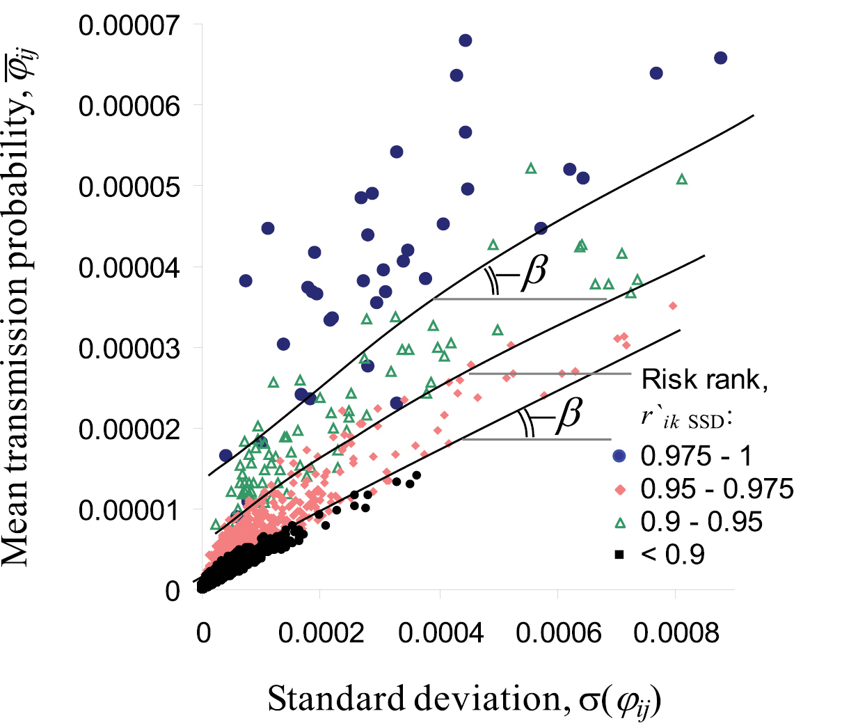
Schematic representation of broad risk classes delineated with the SSD rule, r`ik, in dimensions of the mean camper travel probability, , and its standard deviation, σ(φij). b denotes the tilt angle between the generalized boundaries of broad risk classes in the point cloud - σ(φij) and the horizontal line indicates a constant mean transmission rate (φij = const). Dashed lines denote the boundaries between hypothetical risk classes in a risk-neutral classification (i.e., b = 0, when risk delineation is independent of the amount of uncertainty in the estimates). Points represent individual locations (15×15 km map cells, a 10% random subset of all locations).
Notably, the SSD rule does not restrict the potential range of risk-averse preferences, i.e., it does not limit the degree of decision-makers’ absolute risk-aversion. This suggests that the SSD rule allows for the possibility that the risk aversion of some decision-makers may be very large, such that small differences in the uncertainty of the risk estimates could receive unrealistically high importance. To address instances of extreme risk aversion, several alternative approaches that limit the potential range of risk aversion have been proposed. For example, stochastic dominance with respect to a function (SDRF) limits the range of the absolute risk aversion measure to arbitrary chosen limits (
In economic studies, the SSD rule has commonly been considered too coarse to be used effectively for practical purposes (
In our study, we used the stochastic dominance concept to delineate nested non-dominant sets of map elements, based on a partial order of these elements, in a space defined by the distributions of pest transmission rates φij to a state (province) of interest. The reliance on a partial order of elements makes this approach relatively stable to errors in data and underlying assumptions about the behavior of the invader. Basically, it takes a higher degree of error to alter the partial ordering of elements in the set and change the dominance relations between the map elements.
The stochastic dominance concept (SD) provides an attractive framework for assessing risks of pest invasions under uncertainty. In our study, the theoretical attractiveness of the second-degree stochastic dominance (SSD) lies in its non-parametric nature (
The stochastic ordering techniques used in this study help resolve some troublesome issues in assessing invasion risks when knowledge about an invasive organism is insufficient for deriving precise estimates of risk. A lack of knowledge about the organism’s behavior in a new environment often causes experts to generate fairly coarse assessments (e.g., by assessing risk in vague “high-low” terms or deriving a broad distribution of plausible invasion outcomes instead of a single impact value). Although experts can discern the meaningful tendencies in the predicted outcome of an invasion (such as relatively high or low likelihood of invasion), they are rarely able to assign precise likelihood values. In techniques based on nested non-dominant sets like the FSD and SSD rules, every geographic location of interest is ordered along a risk gradient, which makes the issue of assigning precise pest arrival rate values less critical.
The estimation of non-dominant sets with the FSD or SSD rule requires undertaking multiple pairwise tests for stochastic dominance and has a computational complexity on the order of N(N - 1)/2. While calculation of non-dominant sets for large N can be computationally demanding, the basic algorithm that checks for non-dominance is relatively simple, and can be easily parallelized.
We must note that the use of nested non-dominant sets for ordering geographic locations provides only a partial ranking (so that ranks reflect relative “high-low” positions only within a given dataset). Since our intention was to develop comparable risk rankings derived for the U.S. states, eight Canadian provinces and the Yukon Territory, we undertook the extra step of aggregating all datasets into a single superset and ranking it with the FSD and SSD rules. Thus, the final ranks were mapped within a single frame of reference and the ranks for individual states and provinces were comparable one with another. While computationally demanding we believe this approach addresses a major criticism of risk mapping methods based on a partial ordering: an inability to generate a common ranking space. Table 2 shows a comparative level of risk that each state (or province) will receive infested firewood with recreational travelers as an average rank values, r`ik of firewood moved to a state (or province) of interest from all out-of-state locations as a risk metric. As Table 2 suggests, Texas, Arkansas, and California show the highest potential to receive forest pests in camper-transported firewood from elsewhere, whereas the District of Columbia, Yukon Territory, Nova Scotia, Manitoba and Saskatchewan have the lowest potential. These rankings assume a generalized risk of infestation. Knowledge of a specific potential source location for an infestation could, of course, change these rankings, but the approach used here to incorporate risk aversion in the mapping process would remain applicable.
Incorporation of risk-averse preferences into a delineation of high-risk locations has some important implications for the development of broad-scale pest surveys and public outreach campaigns. In regions where the areas with high-risk estimates based on the SSD rule are uniformly dispersed in relatively close proximity to a state or provincial border (such as for Alabama or Pennsylvania, Appendix 2), the development of large-scale public outreach programs could target nearby states because camper travel is mostly local and risk is distributed uniformly in close proximity to the state (or province) of interest. Alternatively, if the majority of high-ranked source locations indicate long-distance travel destinations (such as for the prominent national parks in Utah or Arizona), a statewide surveillance program may be inefficient and an alternative effort that targets specific high-risk recreation destinations would represent a more effective strategy.
This study demonstrated how the notion of a decision-maker’s risk aversion can be incorporated into the process of mapping risks of ecological pest invasions. We believe that the approach based on the stochastic dominance rules represents a major step forward in model-based assessments of ecological risks because it provides a tractable way to incorporate decision-making preferences into the estimates of pest invasion risk and consecutively offers the appropriate treatment of uncertainty according to the anticipated preferences of decision-makers (the end users of risk assessments and maps). Overall, incorporation of risk-aversion adds credibility to the pest risk mapping process, helps narrow the set of geographical locations that would need to be targeted for costly inspection and public outreach activities, and could be easily applied to the threat of recreational firewood movement in North America.
We thank the Organisation for Economic Co-operation and Development (OECD) Co-operative Research Programme (CRP) on Biological Resource Management for Sustainable Agricultural Systems for sponsoring travel to present this research at the 6th International Pest Risk Mapping Workshop in Tromsø, Norway. We also thank Judith Pasek (USDA APHIS, retired) and David Kowalski (USDA APHIS) for providing the NRRS data and Karen Jamieson (Natural Resources Canada, Canadian Forest Service) for editing the manuscript. The participation of Denys Yemshanov was supported by an interdepartmental NRCan - CFIA Forest Invasive Alien Species initiative. The participation of Mark Ducey was supported by the Agriculture and Food Research Initiative Competitive Grants Program Grant No. 2010-85605-20584 from the National Institute of Food and Agriculture.
Risk of out-of-state (out-of-province) locations to be the source of forest pests transported in firewood carried by campers. The risk rank values are based on the delineation of nested non-dominant sets via the first-degree stochastic dominance rule (FSD). The ranks close to 1.0 denote the highest risk of pest arrival and the ranks close to 0 denote the lowest risk. (doi: 10.3897/neobiota.18.4002.app1) File format: Adobe PDF File (pdf).
Risk of out-of-state (out-of-province) locations to be the source of forest pests transported in firewood carried by campers. The risk rank values are based on the delineation of nested non-dominant sets via the second-degree stochastic dominance rule (SSD), which embeds the notion of risk-averse decision choice. The ranks close to 1.0 denote the highest risk of pest arrival and the ranks close to 0 denote the lowest risk. (doi: 10.3897/neobiota.18.4002.app2) File format: Adobe PDF File (pdf).
Maps of differences in the risk ranks based on the first- and second-degree stochastic dominance rules, Δ r`ik= r`ik FSD – r`ik SSD. Positive values indicate that the FSD-based risk rank exceeds the SSD-based rank and vice versa. (doi: 10.3897/neobiota.18.4002.app3) File format: Adobe PDF File (pdf).
Summary of differences between risk rank classes, 0–0.05, 0.05–0.25, 0.25–0.5, 0.5–0.75, 0.75–0.95 and 0.95–1 in the delineations based on the FSD and SSD rules. (doi: 10.3897/neobiota.18.4002.app4) File format: Adobe PDF File (pdf).