


(C) 2013 Frank H. Koch. This is an open access article distributed under the terms of the Creative Commons Attribution License 3.0 (CC-BY), which permits unrestricted use, distribution, and reproduction in any medium, provided the original author and source are credited.
For reference, use of the paginated PDF or printed version of this article is recommended.
Citation: Koch FH, Yemshanov D, Haack RA (2013) Representing uncertainty in a spatial invasion model that incorporates human-mediated dispersal. In: Kriticos DJ, Venette RC (Eds) Advancing risk assessment models to address climate change, economics and uncertainty. NeoBiota 18: 173–191. doi: 10.3897/neobiota.18.4016
Most modes of human-mediated dispersal of invasive species are directional and vector-based. Classical spatial spread models usually depend on probabilistic dispersal kernels that emphasize distance over direction and have limited ability to depict rare but influential long-distance dispersal events. These aspects are problematic if such models are used to estimate invasion risk. Alternatively, a geographic network model may be better at estimating the typically low likelihoods associated with human-mediated dispersal events, but it should also provide a reasonable account of uncertainties that could affect perception of its risk estimates. We developed a network model that assesses the likelihood of dispersal of invasive forest pests in camper-transported firewood in North America. We built the model using data from the U.S. National Recreation Reservation Service, which document visitor travel between populated places and federal campgrounds across the U.S. and Canada. The study area is depicted as a set of coarse-resolution map units. Based on repeated simulations, the model estimates the probability that each unit is a possible origin and destination for firewood-facilitated forest pest invasions. We generated output maps that summarise, for each U.S. state and Canadian province, where (outside the state or province) a camper-transported forest pest likely originated. Treating these output maps as a set of baseline scenarios, we explored the sensitivity of these “origin risk” estimates to additive and multiplicative errors in the probabilities of pest transmission between locations, as well as random changes in the structure of the underlying travel network. We found the patterns of change in the origin risk estimates due to these alterations to be consistent across all states and provinces. This indicates that the network model behaves predictably in the presence of uncertainties, allowing future work to focus on closing knowledge gaps or more sophisticated treatments of the impact of uncertainty on model outputs.
Human-mediated dispersal, firewood, forest pests, pest risk mapping, network modelling, uncertainty
The spread of invasive alien species is largely facilitated by human activities such as trade and travel (
However, there has been increased recognition of the utility of network-based modelling approaches to depict human-mediated dispersal of invasive species (
In North America, there is increasing concern that forest pest invasions are being facilitated by the transport of firewood for recreational purposes (
Treating these output maps as a set of baseline scenarios, we explored the sensitivity of their “origin risk” estimates to errors in the probabilities of pest transmission between locations, as well as randomized removal of nodes from the underlying network. Here, we discuss the implications of these sources of uncertainty for the interpretation of the derived maps. The use of sensitivity analysis techniques to characterize the influence of uncertainty on model outputs is not unusual (
We constructed our network model using a broad-scale data set from the U.S. National Recreation Reservation Service (NRRS), which operates an online reservation system for campgrounds and related facilities operated by the U.S. Forest Service, National Park Service, Bureau of Land Management, and other federal agencies. The available data spanned a period of greater than five years (January 2004-September 2009) and documented ~7.2 million visitor reservations, including reservations from Canada, at campgrounds and recreational facilities throughout the continental U.S. Although this is a large data set, there are many public and private campgrounds outside the NRRS system. Hence, we assumed the data to be a representative sample of all camper travel.
Each reservation record documented the visitor’s origin location (i.e., by ZIP code or Canadian postal code), the destination campground, and the date of the visit. The initial processing of the NRRS data set is described in greater detail in
For each individual reservation, we calculated the geographic (Euclidean) distance between the visitor’s origin location (i.e., the centroid of the polygon depicting the visitor’s ZIP or postal code) and the destination campground. We then parsed the data into a set of unique pathway segments. Some data aggregation was necessary during this step to ensure model tractability. Conceptually, our network model is formulated as a first-order transition matrix (
Any two map cells, designated i and j, in this networked set were connected by a unique pathway segment, ij. Each ij had a value, mij, representing the number of trips from i to j documented in the aggregated NRRS data during the study time period t (i.e., January 2004-September 2009), and another value, mji, representing the number of return trips from j back to i. We constructed a matrix, M, from these mij and mji values. The size of the matrix was n × n, corresponding to the number of unique map units in the aggregated data (i.e., n = ~14, 000):
 (1)
(1)
The non-diagonal elements of M were the mij and mji values for the pathway segments connecting each (i, j) pair of map cells. The diagonal elements of M, where i = j, were set to 0.
Based on M, we constructed a probability matrix, Pt, of camper travel (and by extension, transport of potentially infested firewood) along the pathway segments during the study period t. We assumed that the probability, pij, of travel along any given segment ij was linearly related to the number of trips from i to j during period t:
pij = mij λt, (2)
where λt is a scaling parameter. Ideally, the parameter λt would define the total likelihood (i.e., over the study period t) of camper transport of pest-infested firewood from i to j in the pathway matrix. In fact, a precise value of λt would be necessary to estimate an exact probability of a pest being moved from location i to j. Our objective, however, was not to derive exactly estimated output probabilities, but the more conservative goal of testing the relative sensitivity of model outputs to changes in the inputs, such that the output probabilities simply serve as a relative measure of risk. For this purpose, we only needed λt to be sufficiently small to ensure that the sum of the pij probabilities in each Pt matrix row was below 1.
Each row of Pt included another variable, pi term, representing the probability that no camper travel (i.e., to any j) would originate at i:
 (3)
(3)
If pi term was equal to 1 for any row, then the map cell i associated with that row did not serve as a point of origin in the model. This did not preclude the cell from serving as a potential destination j. The probability matrix Pt of camper travel along each pathway segment (i.e., during period t) was thus specified as follows:
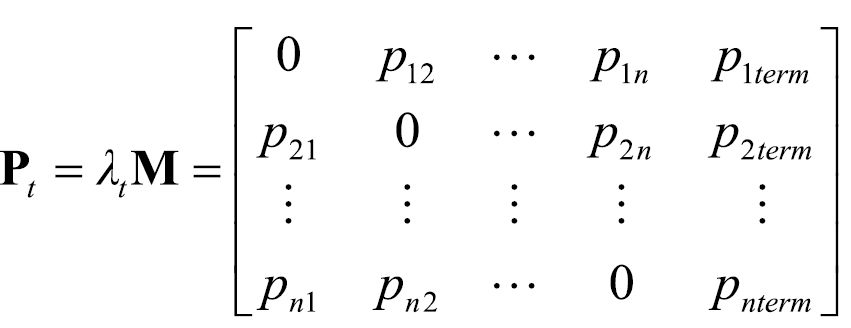 (4)
(4)
We used Pt as the basis for 2 × 10⁶ stochastic pathway simulations of camper travel from each cell i to other map cells. Setting i as the origin location, the model extracted the vector of travel probabilities associated with i (i.e., the probabilities in row i) from Pt in order to simulate subsequent camper travel from i through the pathway network to other map cells. Briefly, in each simulation run for a given cell i, the model performed a uniform random draw against the associated row of probabilities in Pt in order to select the next map cell defining the path of an individual trip. The simulation of this path continued until reaching a final destination map cell (i.e., a cell with no outgoing travel), or instead, when a terminal state (i.e., no further travel) was selected based on the pi term value. Regardless of the number of individual segments comprising a simulated path, we assumed that the path was completely traversed within the study period t. Consequently, for a given pathway segment ij, the probability of camper travel from location i to location j during period t was estimated as follows:
φij = Mij/M, (5)
where Mij is the number of times pathway travel from location i to j was simulated to occur, and M is the total number of simulations (M = 2 × 10⁶ in this study).
The network model permitted us to generate maps where each individual cell in the study area could be set as the origin or destination location of interest. While cell-specific maps might have value when addressing specific invasion scenarios (e.g., identifying the probable source locations for a single cell found to be invaded), they do not provide a comprehensive picture of invasion risk for use in setting management priorities. So, we chose to summarize the model results in a broader context. In a previous analysis of the NRRS data (
For each U.S. state and Canadian province, we generated a map where, for each cell i outside the target state (province), we summed the model-derived travel probabilities (i.e., the φij values) for all pathways between i and any destination cell j within the target state (province). Essentially, each map depicts the most likely external source locations if a firewood-transported forest pest were to be discovered within the state (province) of interest. (Note that for the Canadian provinces, we assume that campers returning from U.S. locations may be transporting forest pests, despite border biosecurity measures.) A principal feature of these maps is that they highlight key “bottleneck” locations where surveillance, awareness campaigns, or quarantine procedures have the best potential to be cost-effective in terms of protecting the state (province) of interest from invasion (
We performed sensitivity analyses to evaluate how uncertainty in key aspects of the network model’s structure would influence the φij probabilities estimated in the baseline maps. The primary goal of these analyses was to assess whether uncertainties in any of the tested model aspects yielded a set of output maps with spatial patterns that departed in unexpected ways from the patterns depicted in the corresponding baseline maps. We adopted a Monte Carlo simulation approach (
We focused on three model aspects for this study. Our first sensitivity scenario tested the impact of uncertainty in the network configuration by randomly removing up to 30% of nodes (i.e., map cells and their associated vectors of pij probabilities) from the network prior to each new model run. Our second sensitivity scenario tested the impact of uncertainty in the scaling parameter λt (see Eq. 2). In this case, we added uniform random error within the range ±0.15 to λt prior to completing each new model run. Our final sensitivity scenario evaluated the impact of uncertainty in the pij values comprising Pt. To test this aspect, we added uniform random error of up to 0.01 to the pij values before each new model run. Ideally, we would have repeated the three scenarios with series of bounding values. However, because of the computational complexity of this exercise, we chose a single bounding value for each sensitivity scenario that, based on preliminary work with the model, we were confident would provide meaningful contrast to the baseline scenario.
We completed 2 × 10⁶ pathway simulations for each sensitivity scenario. This process yielded scenario-specific maps of the φij probabilities (see Eq. 5) for each state and province that we could compare to the corresponding baseline maps. For this comparison, we calculated and mapped the differences, in percentage terms, between the output probabilities under the baseline scenario and under each sensitivity scenario. We also calculated a Moran’s I (
We employed a simple rank-difference approach for further comparison of the baseline results to those from our third sensitivity scenario dealing with uncertainty in the pij values. After calculating the per-cell differences between the baseline and sensitivity maps for each state and province, we converted both the baseline probabilities and the calculated differences into ranks. Each cell in a given map was assigned a rank from 1 to 6 based on a global percentile distribution of the values that occurred in the maps for all states and provinces; cell values that fell within the bottom 25% of this global distribution received a rank of 1, cells in the 25–75% range received a rank of 2, cells in the 75–90% range received a rank of 3, cells in the 90–95% range received a rank of 4, cells in the 95–99% range received a rank of 5, and cells in the top 1% of this distribution received a rank of 6. We ranked each cell twice in this fashion, first according to its percentile value under the baseline scenario, then according to its percentile value in the global distribution of differences under this sensitivity scenario. Next, we calculated the change in rank between the two, which yielded an index value ranging from -5 to 5. Finally, we mapped the index values for each state and province in order to identify any spatial trends.
Across all individual state and province maps created for the baseline scenario, we saw three general spatial patterns of out-of-state (or out-of-province) origin risk. First, as illustrated by the state of Alabama (Fig. 1a), there were cases where the highest origin probabilities (i.e., the per-cell φij values) were primarily limited to a narrow fringe zone surrounding the target state. This pattern was common among states in the southeastern and northeastern U.S. The second general pattern, exemplified by Missouri (Fig. 1b), similarly featured a localized zone of high probabilities around the target state, but this was augmented by several high-probability hotspots associated with major urban areas located outside this zone. For instance, the map for Missouri included hotspots associated with the cities of Chicago (IL), Dallas (TX), Denver (CO), all of which are at least 400 km away. This mixed origin pattern was typical of many states in the U.S. Midwest. In the third pattern, exemplified by Utah (Fig. 1c), there was also a subtle local fringe zone, but the majority of map cells with high probabilities were associated with major urban areas that are fairly distant from the target state. With respect to Utah, the most prominent urban areas (i.e., those displaying uniformly high probabilities) were generally in the western U.S., but a number of eastern U.S. cities also had probabilities in the top 5% of the global distribution of probabilities across all states and provinces. This sort of dispersed pattern of origin risk was exhibited by other states such as Arizona and California that, like Utah, feature several popular recreational destinations (e.g., national parks) that draw campers from throughout the continent.
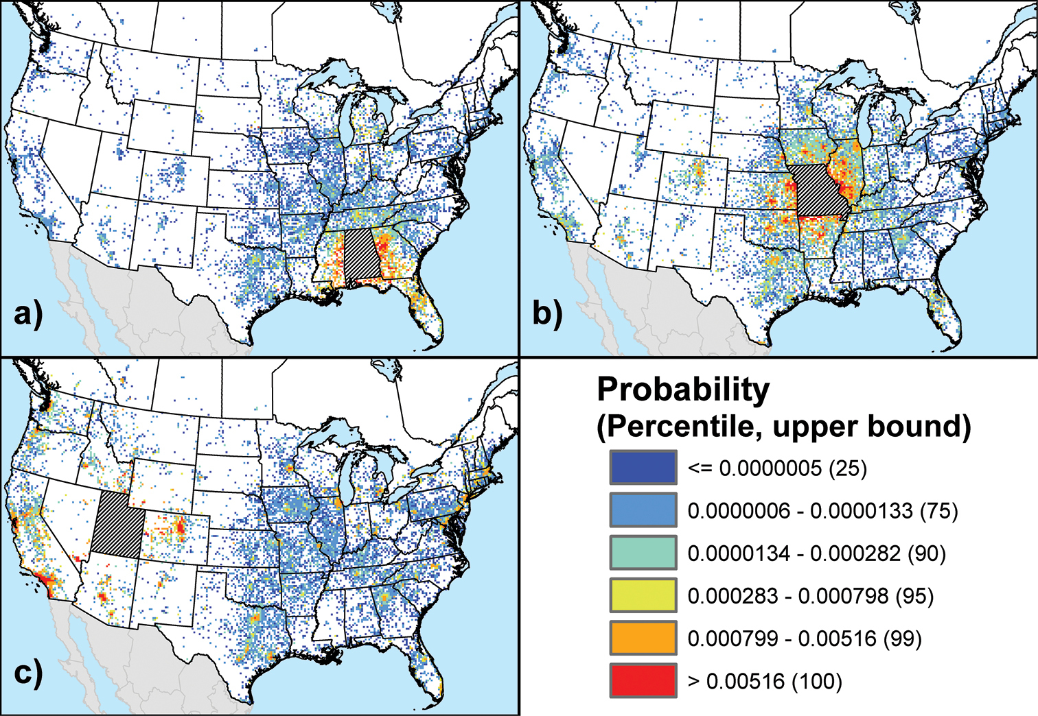
Out-of-state origin risk maps for three U.S. states under the baseline scenario: a Alabama b Missouri c Utah. The maps show the relative probability, φij, that a map cell outside the state of interest is a source of campers carrying potentially infested firewood to the target state. Numbers in parentheses link the defined probability classes to a global percentile distribution built from the probabilities that occurred in the maps for all states and provinces.
The maps for the Canadian provinces, especially the more populous ones (i.e., Quebec, Ontario, Alberta, and British Columbia), usually exhibited a dispersed spatial pattern similar to that observed for Utah, although the origin probabilities in each map were low compared to their U.S. counterparts. Indeed, the highest probabilities in these maps very rarely reached the top 10% of the global distribution. The only exceptions were a few high-probability (top 5%) cells in each of the maps for the most populous Canadian provinces, which appeared to be associated with specific recreational destinations such as Grand Canyon National Park (AZ) and Zion National Park (UT).
Two factors seem to govern the observed patterns of origin risk. Foremost is the population of the state or province of interest. Because the model is bi-directional (i.e., it also simulates return travel by campers from their destinations to their origin locations), the population of the target state or province influences the range of output probabilities that will be portrayed in its map, particularly the frequency at which high probabilities occur. In short, the maps of heavily populated states and provinces tended to have higher probabilities overall than sparsely populated states and provinces. The second factor is the nature of the recreational opportunities available in the target state or province. States or provinces containing several high-profile recreational destinations displayed a dispersed pattern of origin risk, while states or provinces with numerous but comparatively low-profile recreational destinations usually displayed a more localized origin risk pattern.
Figure 2 shows three example maps of the mean percent difference (i.e., over all model runs) in the φij output probabilities under this sensitivity scenario. The example states correspond to those highlighted under the baseline scenario: Alabama (Fig. 2a), Missouri (Fig. 2b), and Utah (Fig. 2c). Note that only map cells in the top 10% of probabilities under the baseline scenario are shown. For all states and provinces, the percent change in the values of cells in this top 10% typically ranged from -24% to -36%, with a map-wide mean (i.e., across all cells in a given map) near -30%. This level of difference is consistent with the proportion of nodes removed for this scenario. More importantly, as illustrated by the difference maps for all three example states, there was no obvious spatial trend in the pattern of change. Essentially, each map has a salt-and-pepper appearance, such that cells with higher probabilities under the baseline scenario (see Fig. 1) do not appear to have greater (or smaller) percent changes than cells with lower probabilities under the baseline. This observation is supported by the Moran’s I values calculated for all states and provinces, which ranged between -0.016 and 0.021 (median = 0.005) and thus indicated a minimal level of spatial autocorrelation.

Maps of the mean percent difference (i.e., across all model runs) between the φij output probabilities calculated under the baseline scenario and under the sensitivity scenario that tested the impact of uncertainty in the network configuration: a Alabama b Missouri c Utah. Only cells with probabilities in the top 10% of the global distribution for the baseline scenario are shown.
Figure 3 shows three example maps of the mean percent difference in the φij output probabilities under this sensitivity scenario. As in the previous scenario, the example states correspond to those highlighted under the baseline scenario: Alabama (Fig. 3a), Missouri (Fig. 3b), and Utah (Fig. 3c). Only map cells in the top 10% of probabilities under the baseline scenario are shown. For all states and provinces, the percent change in the values of cells in this top 10% typically ranged from -15% to 15%, with a map-wide mean slightly greater than 0. This degree of change is consistent with the alterations to λt under this scenario.
None of the difference maps for the example states appears to show a strong spatial trend in the pattern of change. There may be a slight tendency for map cells with higher probabilities under the baseline scenario to exhibit small but positive percent changes, while cells with lower probabilities under the baseline may tend toward small negative changes. However, the existence of a subtle spatial trend is not really supported by the Moran’s I values for each state and province, which ranged from -0.005 to 0.133 (median=0.008). Indeed, with the exception of a single Canadian province, Nova Scotia, which has relatively few connections to outside locations in our network model, none of the maps had an I value greater than 0.0324. Similar to the previous sensitivity scenario, this suggests a low level of spatial autocorrelation.
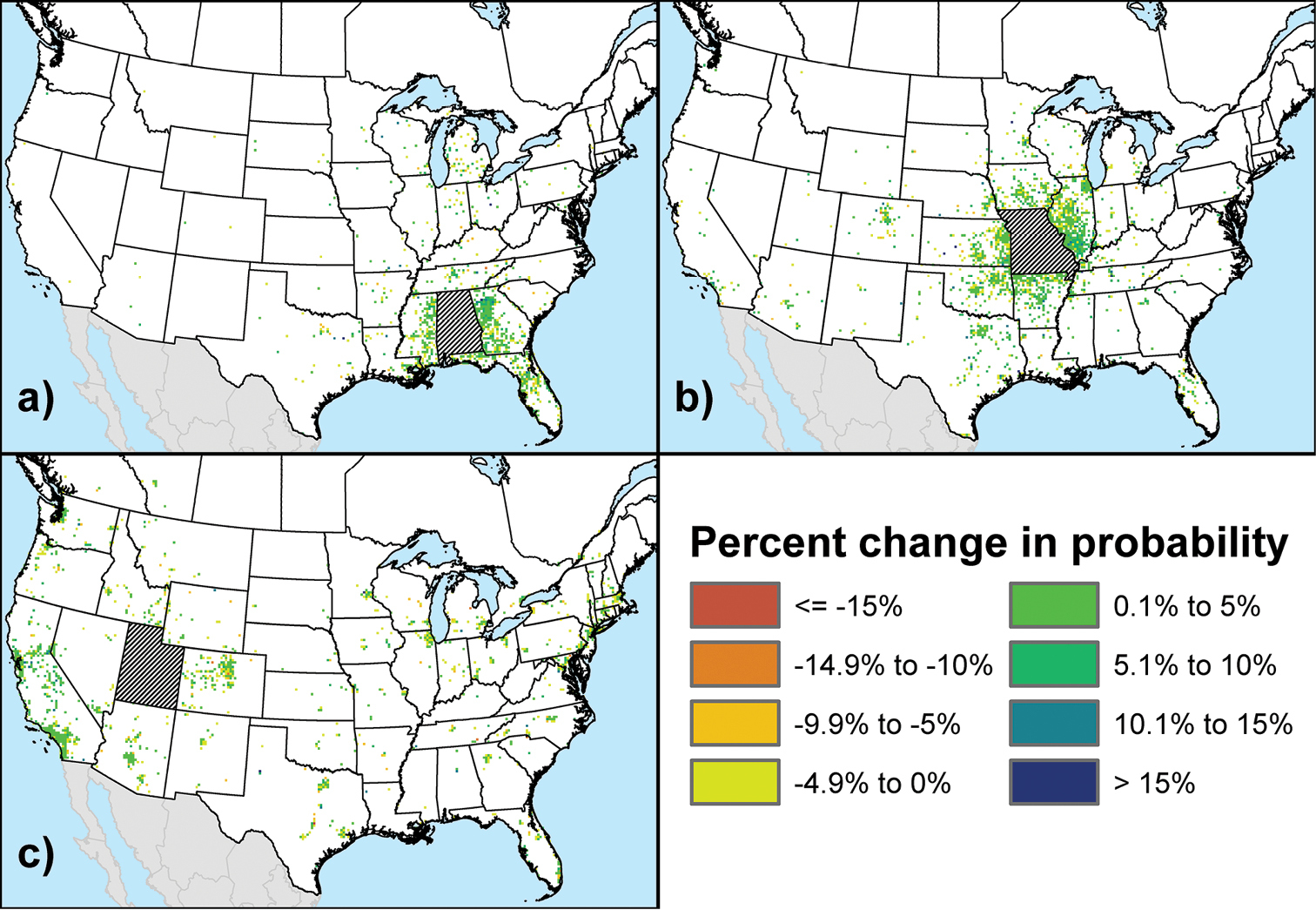
Maps of the mean percent difference (i.e., across all model runs) between the φij output probabilities calculated under the baseline scenario and under the sensitivity scenario that tested the impact of uncertainty in the scaling parameter λt: a Alabama b Missouri c Utah. Only cells with probabilities in the top 10% of the global distribution for the baseline scenario are shown.
Figure 4 shows three example maps of the rank differences (see Methods) between the baseline scenario and this sensitivity scenario, which tested the effects of adding uniform random error to the pij probabilities. The maps display an obvious spatial trend in the pattern of change. (Again, only cells in the top 10% of probabilities under the baseline scenario are shown.) This trend can be summarized in general terms: cells with comparatively higher probabilities under the baseline scenario were more likely to exhibit a decrease or no change in rank under this sensitivity scenario, while cells with comparatively lower probabilities under the baseline were more likely to exhibit an increase in rank. Thus, for states and provinces like Alabama (Fig. 4a), where the highest origin probabilities under the baseline scenario were primarily limited to a localized zone adjoining the state or province (also see Fig. 1a), any decreases in rank were also usually limited to this zone. Alternatively, in states and provinces like Missouri (Fig. 4b) and Utah (Fig. 4c), where high origin probabilities under the baseline were regularly associated with major urban areas outside the fringe zone, it is primarily map cells in these areas that exhibited a decrease or, just as commonly, no change in rank. For all states and provinces, the map cells that exhibited increases in rank under this sensitivity scenario were usually found in rural areas or the peri-urban zones (
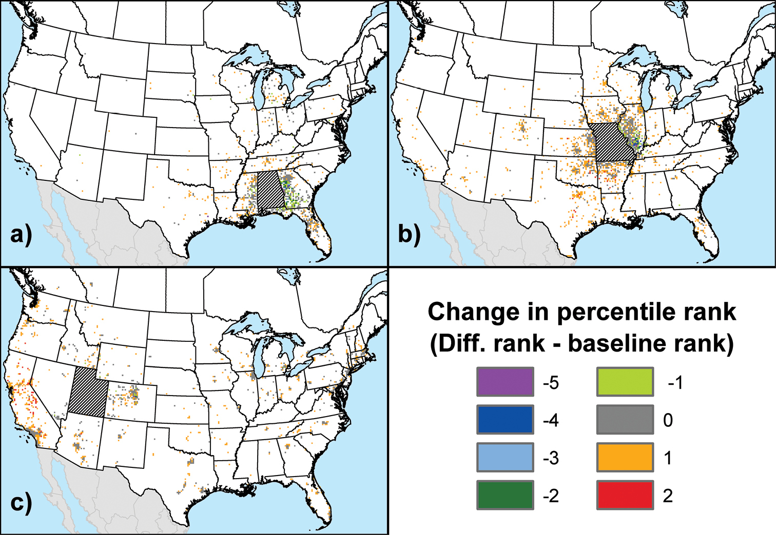
Maps showing the difference in rank between maps generated under the baseline scenario and under the sensitivity scenario that tested the impact of uncertainty in the pij probabilities: a Alabama b Missouri c Utah. See main text for details regarding the calculation of ranks, which ranged from 1 to 6 for each scenario. Only cells with probabilities in the top 10% of the global distribution for the baseline scenario are shown.
The existence of a spatial trend in the pattern of change is supported by the Moran’s I values calculated for the difference maps of each state and province. With the exception of Nova Scotia, the values ranged from 0.057 to 0.208 (median = 0.135), indicating a degree of positive spatial autocorrelation (i.e., clustering) that varied according to whether the state or province of interest had a well-defined fringe zone of high probabilities under the baseline scenario. Typically, states and provinces with such a zone exhibited larger I values. This variability, however, does not contradict the notion of a generally consistent spatial trend across all states and provinces.
By focusing on changes in the φij probabilities under the sensitivity scenarios, we can make conclusions about how the model generally behaves given uncertainty in the tested model aspects. We expected to see departures from the baseline φij values in all three scenarios, but importantly, our results indicated that the patterns of these differences were consistent across all states and provinces. In the two scenarios testing the impact of uncertainty in the network configuration and in the scaling parameter λt, the distribution of the mapped differences was usually close to random; in other words, no particular state (province) or range of output probabilities was uniquely affected by uncertainty in these model aspects. In the scenario that tested the impact of uncertainty in the pij values, there was a recognizable spatial trend in the differences from the baseline scenario, but this trend was manifested similarly across all states and provinces. Essentially, uncertainty in the pij values resulted in smoothing of the φij output probabilities across the entire map area, regardless of how those probabilities were spatially distributed under the baseline scenario.
In summary, it appears that the network model is generally stable in the presence of uncertainties in its critical structural aspects (i.e., in its spatial configuration and in parameters that define Pt, the probability matrix that drives the pathway simulations). While making this determination was the primary objective of our study, close examination of the individual sensitivity scenarios reveals additional details about potential model improvements and future applications. First, removing a large portion of the nodes from the network did not cause the model to behave inconsistently. This stability suggests that the modelling framework may be transferable to other data sets that can be organized as networks, including potentially sparser data sets. This transferability may present an easy opportunity to examine other modes of human-mediated dispersal that are relevant to invasion risk. For instance, we might want to apply the model to describe camper travel patterns associated with privately owned campgrounds across North America. The framework may also be applicable to the movement of crop pests via domestic shipments of certain agricultural commodities. Similarly, the network model continued to behave consistently despite sizeable alterations to the scaling parameter λt. This appears to affirm our supposition that a more precise value for λt would not substantially affect the generalbehaviour of the model, which further supports the notion of its transferability to other invasion risk modelling problems.
In the sensitivity scenario that tested the impact of uncertainty in the pij probabilities, the smoothing effect observed in the output maps suggests that these probabilities were fairly sensitive to uncertainty, or at least more sensitive than the other tested model aspects. Under this scenario, a small random variate was added to every pij value in the Pt matrix, including where pij = 0. This change effectively created new interconnecting vectors between network nodes, subsequently adding topological information to the network. Indirectly, this raised the relative importance of map cells with low origin probabilities under the baseline scenario, since it added some small probability of camper travel between cells, even in cases where no such travel was documented in the NRRS data.
Conceptually, this sensitivity scenario depicts a general lack of knowledge about the travel patterns of campers (and by extension, their movement of potentially infested firewood). This implies that the best opportunity to improve our model may be to refine the pij probabilities. Notably, these values are partly shaped by the parameter λt (see Eq. 2), so the issues mentioned previously regarding λt may have relevance here. Indeed, while we did not implement a sensitivity scenario where λt and the pij values were varied together, it is possible that the pij values are more or less sensitive depending on the value of λt. This is a potential topic of future work. Regardless, the pij values are directly derived from the data underlying the network, and so depend on the comprehensiveness and representativeness of those data for the phenomenon being modelled. In our case, the NRRS data only cover a limited subset of all camper travel, so there could be some advantage to including other data sources such as camper reservation records at private- or state/provincial-managed campgrounds, contingent on the availability of such data.
We must reiterate that the φij output probabilities only provide a relative measure of invasion risk. Because we did not have sufficient data to directly model the movement of forest pests in infested firewood, and instead modelled the travel of all campers as a proxy, then the resulting probabilities should not be interpreted as a depiction of the true risk. The actual probabilities of successful forest pest introduction via firewood are likely much lower than the numbers we present here, for various reasons; for instance, not all campers transport firewood, not all of the firewood they transport is infested, and not all infested firewood contains enough individuals of a potential pest species to support establishment upon arriving at a destination (
While we have proposed that network models may be especially useful for mapping pest risk, they, like other types of models, should be subject to critical scrutiny prior to their application. We see the presented approach as being primarily of interest to analysts tasked with constructing network models. The approach does not address key questions that arise in uncertainty analysis regarding how uncertainty propagates to the model outputs, or the resulting implications for decision makers who will utilize these outputs. Instead, it is merely intended to help analysts assess the fundamental soundness of their models and feel more confident about incorporating them into their analytical toolsets.
Because human activities contribute significantly to the proliferation of invasive species, modelling approaches that characterize important human-mediated dispersal pathways may be highly applicable for pest risk analysis. To provide a working example, we developed a geographically explicit network model that depicts the potential spread of forest pests in firewood moved by camper travel across the U.S. and Canada. We then presented an approach, based on common sensitivity analysis techniques, for assessing how this network model behaves when uncertainty is introduced into critical model aspects. In our case, the approach allowed us to determine that the model behaved consistently and predictably in the presence of uncertainty. The approach is analytically straightforward, and should be generalisable to other network models with comparable formulations.
We thank Judith Pasek (USDA APHIS, retired) and David Kowalski (USDA APHIS) for providing the NRRS data, as well as Roger Magarey (North Carolina State University) and Daniel Borchert (USDA APHIS) for their assistance with the project. The participation of Denys Yemshanov was supported by an interdepartmental NRCan - CFIA Forest Invasive Alien Species initiative.