


(C) 2013 David Makowski. This is an open access article distributed under the terms of the Creative Commons Attribution License 3.0 (CC-BY), which permits unrestricted use, distribution, and reproduction in any medium, provided the original author and source are credited.
For reference, use of the paginated PDF or printed version of this article is recommended.
Citation: Makowski D (2013) Uncertainty and sensitivity analysis in quantitative pest risk assessments; practical rules for risk assessors. In: Kriticos DJ, Venette RC (Eds) Advancing risk assessment models to address climate change, economics and uncertainty. NeoBiota 18: 157–171. doi: 10.3897/neobiota.18.3993
Quantitative models have several advantages compared to qualitative methods for pest risk assessments (PRA). Quantitative models do not require the definition of categorical ratings and can be used to compute numerical probabilities of entry and establishment, and to quantify spread and impact. These models are powerful tools, but they include several sources of uncertainty that need to be taken into account by risk assessors and communicated to decision makers. Uncertainty analysis (UA) and sensitivity analysis (SA) are useful for analyzing uncertainty in models used in PRA, and are becoming more popular. However, these techniques should be applied with caution because several factors may influence their results. In this paper, a brief overview of methods of UA and SA are given. As well, a series of practical rules are defined that can be followed by risk assessors to improve the reliability of UA and SA results. These rules are illustrated in a case study based on the infection model of
Model, Pest risk assessment, Sensitivity, Uncertainty
Different types of mathematical models are commonly used for pest risk analysis. Some models are used for calculating probability of entry (e.g.,
Uncertainty and sensitivity analysis are two techniques for evaluating models. Although both techniques are often mixed together, they each have a different purpose. Uncertainty analysis (UA) comprises a quantitative evaluation of uncertainty in model components, such as the input variables and parameters for a given situation, to determine an uncertainty distribution for each output variable rather than a single value (
The use of formal uncertainty analysis was recently considered as one of the most important accomplishments in risk analysis since the 1980s (
The main purpose of sensitivity analysis (SA) is to determine how sensitive the output of a model is with respect to elements of the model subject to uncertainty. The objective of a sensitivity analysis is to rank uncertain inputs according to their influence on the output. Sensitivity analysis can be seen as an extension of uncertainty analysis. Its purpose is to answer the following question “What are the most important uncertain inputs?”. Sometimes, SA is also used for a more general purpose such as to understand how the model behaves when some input or parameter values are changed.
Uncertainty and sensitivity analysis are becoming more popular, especially due to development of Bayesian methods and of specialized software and packages (e.g., the sensitivity package of R). However, these techniques should be applied with caution because several factors may influence their results (
For some simple models, it is possible to calculate the exact probability distribution of the model output from the probability distributions of the uncertain input variables and/or parameters. However, in most cases, it is not possible to calculate the probability distribution analytically and other methods should be used. One method is to linearize the model from its derivatives in other words the derivatives of the model output with respect to its inputs and parameters. If the uncertain factors are all assumed normally distributed, then it is possible to estimate the probability distribution of the linearized model analytically which is a normal distribution whose mean and variance are functions of the means and variances of the uncertain factors. A limitation of this method is that its application is restricted to the cases where the uncertain factors are in fact normally distributed. It is sometimes more appropriate to use other distributions, especially when the random variables are discrete or when they are bounded. Another limitation is that this method can be unreliable when the linear approximation is not accurate. For these reasons, the use of a four-step method, based on Monte Carlo simulations, adapted from
Step 1. Define probability distributions for the uncertain model inputs and parameters
The uncertainty about a quantity of interest is frequently described by defining this quantity as a random variable. Uncertainty about model parameter/input values can be described using different types of probability distributions. The uniform distribution, which gives equal weight to each value within the uncertainty range, is commonly used when the main objective is to understand model behavior, but more flexible probability distributions are sometimes needed to represent the input and parameter uncertainty. When the model input corresponds to a discrete variable, for example, the number of imported consignments, or number of successful incursions, discrete probability distributions such as the Poisson are often appropriate (e.g.,
In some cases, it is difficult to define reliable probability distributions for all uncertain model inputs, i.e., probability distributions correctly reflecting the current state of knowledge about input values based on available data and expert knowledge. In such cases, it is useful to define several probability distributions and, when possible, to run the analysis for all of them and to compare the results. This method is illustrated in the example below. When the computation time is too long or when it is not possible to run the analysis several times with different distributions, it is important to present the assumptions explicitly, and to acknowledge that the results of the analysis may have been different if other probability distributions had been defined.
Step 2. Generate values from the distributions defined at step 1
Simple random sampling is a popular method for generating a representative sample from probability distributions. This sampling strategy provides unbiased estimates of the expectation and variance of random variables. Other sampling techniques like Latin hypercube can also be used, especially when the number of variables is large. It is also possible to generate combinations of values of uncertain factors by using experimental designs, for example, complete factorial designs. The latter technique was used by the
Step 3. Compute the model output(s) for each generated input set
Once the parameter/input values have been generated, the next step consists of running the model for each unique set of parameter/input values. For example, if N was set equal to 100, the model must be run 100 times leading to 100 values per output variable. This step may be difficult when computation of model output is time-consuming and, with some very complex models, the value of N must be set equal to a small value due to computation time constraints. This third step will be easier with more simple and less computationally intensive models.
Step 4. Describe the distributions of the model outputs
The distribution of the model output values generated at step 3 can be described and summarized in a number of ways. It is possible to present the distribution graphically using, for example, scatterplots, histograms, density plots. It is also useful to summarize the distribution of the model output values by its mean, median, standard deviation, and quantile values. All these techniques have been applied in several quantitative risk assessments (e.g.,
Sensitivity analysis can be seen as an extension of uncertainty analysis. It comprises computing sensitivity indices to rank uncertain input variables or parameters according to their influence on the model output. Two types of sensitivity analysis are usually distinguished: local sensitivity analysis and global sensitivity analysis (
A sensitivity index is a measure of the influence of an uncertain quantity on a model output variable. Model inputs and parameters whose values have a strong effect on the model are characterized by high sensitivity indices. Less influential quantities are characterized by low sensitivity indices. Thus, sensitivity indices can be used to rank uncertain inputs and parameters, and identify those that deserve more accurate measurements or estimation. A large number of global SA methods are available, for example, ANOVA, correlation between input factors and model outputs, methods based on Fourier series, and methods based on Monte Carlo simulations (
In this section, we present a simple example to show how uncertainty and sensitivity analysis can be used in practice. We consider the simple generic infection model for foliar fungal plant pathogens defined by
and
 if
if  and zero otherwise
where T is the mean temperature during wetness period (°C), W is the wetness duration required to achieve a critical disease intensity (5% disease severity or 20% disease incidence) at temperature T. The model output is W and it is computed as a function of the input T. Tmin, Topt, Tmax are minimum, optimal, and maximum temperature for infection respectively, Wmin and Wmax are minimum and maximum possible wetness duration requirement for critical disease intensity respectively. This model was used to compute the wetness duration requirement as a function of the temperature for many species and was included in a disease forecast system (
Tmin, Topt, Tmax, Wmin, and Wmax are five species-dependent parameters whose values were estimated from experimental data and expert knowledge for different foliar pathogens (e.g.,
In this case study, uncertainty and sensitivity analysis techniques were applied to the model defined above for infection of citrus by the fungal pathogen Guignardia citricarpa Kiely. According to
Three series of probability distributions were defined from Table 1:
- Independent uniform distributions (with lower and upper bounds set equal to the values reported in Table 1)
- Independent triangular distributions (with lower and upper bounds set equal to the values reported in Table 1, and the most likely values set equal to the medians of the uncertain ranges)
- Triangular distributions with positive correlation between Tmin and Topt. Values of Tmin were first sampled from the triangular distribution defined in ii. Values of Topt were then generated by adding values sampled from a uniform distribution (14, 16) to the values of. With this method, Topt values were always higher than 24°C and lower than 31°C, and were correlated to Tmin. The parameter Topt does not follow a triangular distribution anymore, but the other parameters are still distributed according to the triangular distributions defined in ii.
These probability distributions were based on the same information; the lower and upper bounds defined for each model parameter in Table 1. Nonetheless, these distributions describe uncertainty in different ways; the triangular distribution gives higher weights to values located in the middle of the range, and the last distribution considers that two parameters out of five are not independent.
Uncertainty ranges of the five model parameters for Guignardia citricarpa Kiely
| Parameter | Lower bound | Upper bound |
|---|---|---|
| (°C) | 10 | 15 |
| (°C) | 25 | 30 |
| (°C) | 32 | 35 |
| (h) | 12 | 14 |
| (h) | 35 | 48 |
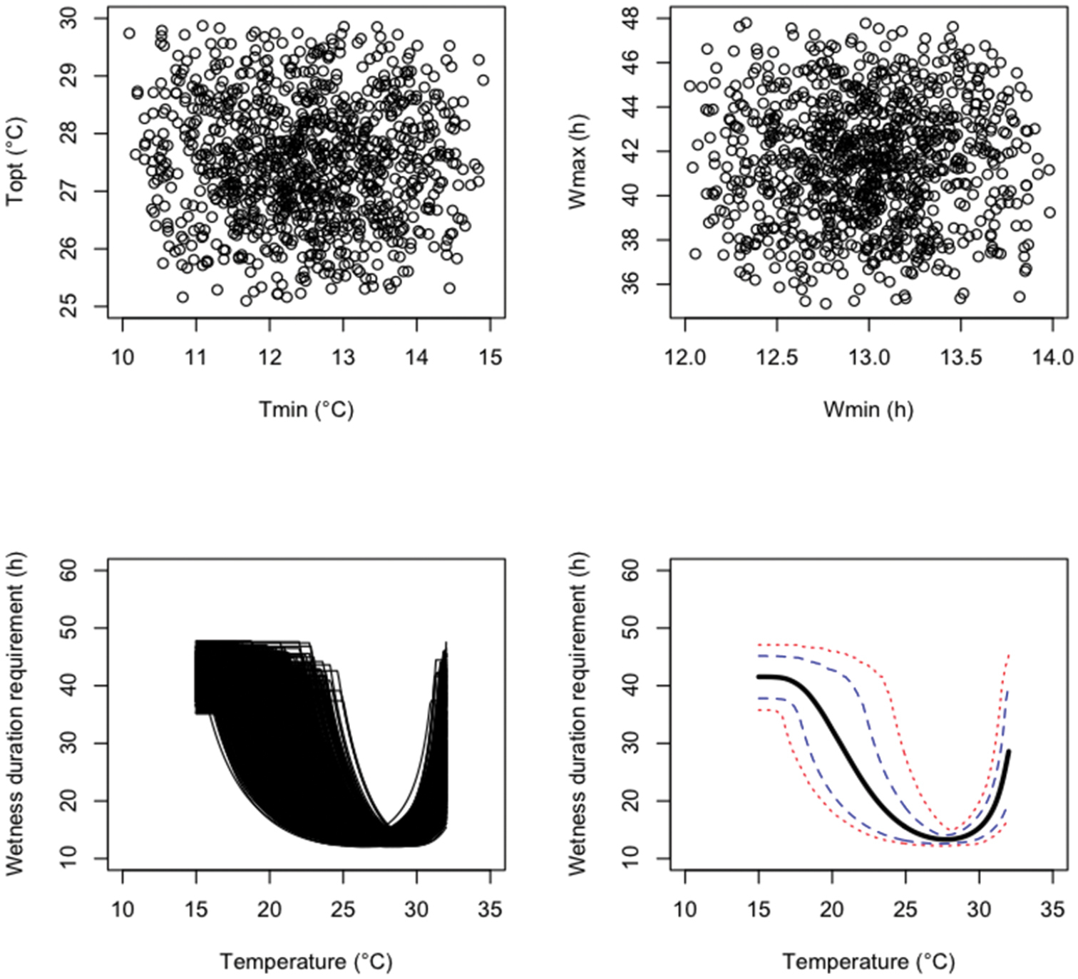
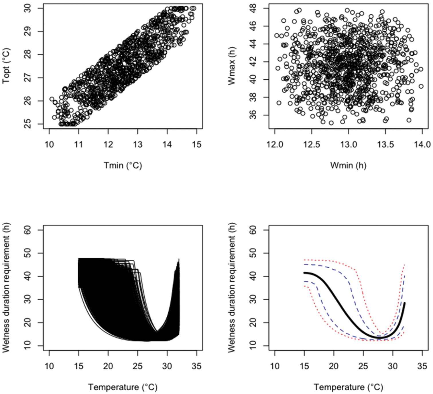
An uncertainty analysis was performed by generating N=1, 000 parameter values from the three probability distributions defined above successively. Results are presented in Figures 1 (probability distribution i), 2 (probability distribution ii), and 3 (probability distribution iii). The sampled parameter values are more concentrated in the central parts of their uncertainty ranges with the independent triangular distributions (Figure 2) than with the independent uniform distributions (Figure 1). Figure 3 clearly shows that, with distribution iii, Tmin and Topt were positively correlated. The 99%, 90% 10% and 1% percentiles and mean values of the model output W reported for different temperatures show that, with all probability distributions, uncertainty about fungus wetness duration requirement is quite small if the temperature is close to 27–28 °C, but much larger for temperature below 25 or above 32 (Figures 1–3). Uncertainty about the wetness duration requirement is reduced with the triangular distribution (Figure 2) compared to the uniform (Figure 1).
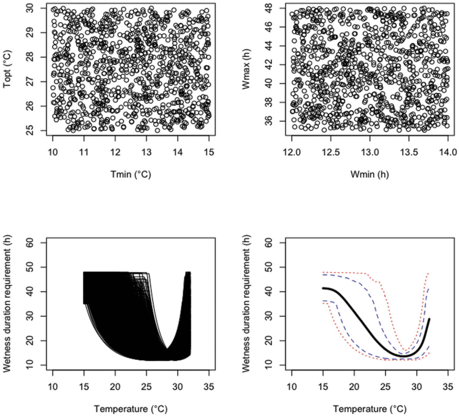
Results of an uncertainty analysis performed with 1, 000 Monte Carlo simulations. The upper graphics show the values of four model parameters sampled from uniform distributions. The lower graphics show the resulting distribution of model outputs, their means (think black line), 10 and 90% percentiles (dashed lines), and 5 and 95% percentiles (dotted lines).
Results of an uncertainty analysis performed with 1, 000 Monte Carlo simulations. The upper graphics show the values of four model parameters sampled from independent triangle distributions. The lower graphics show the resulting distribution of model outputs, their means (think black line), 10 and 90% percentiles (dashed lines), and 5 and 95% percentiles (dotted lines).
Results of an uncertainty analysis performed with 1, 000 Monte Carlo simulations. The upper graphics show the values of four model parameters sampled from triangle distributions assu- ming a positive correlation between Tmin and Topt. The lower graphics show the resulting distribution of model outputs, their means (think black line), 10 and 90% percentiles (dashed lines), and 5 and 95% percentiles (dotted lines).
A sensitivity analysis was performed using the Morris method to identify the most influential parameters of the model. The method of Morris is frequently used to quickly screen among all uncertain inputs (
- Define a design by combining k values of the p uncertain parameters
- Add a small incremental step Δ to one uncertain parameter zi
- Compute an “elementary effect” defined by
![]()
where y() is the model function and z1, ..., zp are the p uncertain parameters - Repeat the procedure several times for all uncertain parameters
- Compute the mean and variance of elementary effects from r replicates. A high mean indicates a parameter with an important influence on the output. A high variance shows that the elementary effect is highly dependent on the value of the uncertain parameter. It indicates either a parameter interacting with another parameter or indicates a parameter whose effect is non-linear. The tuning parameters of the Morris method were set equal to the following values: k=4, p=5, Δ=2, and r=100. The lower and upper bounds of the model parameters were set equal to the values reported in Table 1. Note that it was implicitly assumed here that the uncertain model parameters were uniformly distributed.
Figure 4 shows the mean and the standard deviation of the elementary effect computed using k=4, p=5, Δ=2, and r=100. Results show that the two most influential parameters are Tmax and Topt. The high standard deviations obtained for both parameters reveals the existence of either strong nonlinear effects or strong interactions between the two parameters. This result shows that the effects of a change of Tmax and Topt on wetness duration requirements depend on the values of these parameters (non linearity) and/or on the values of the other parameters of the model (interaction).
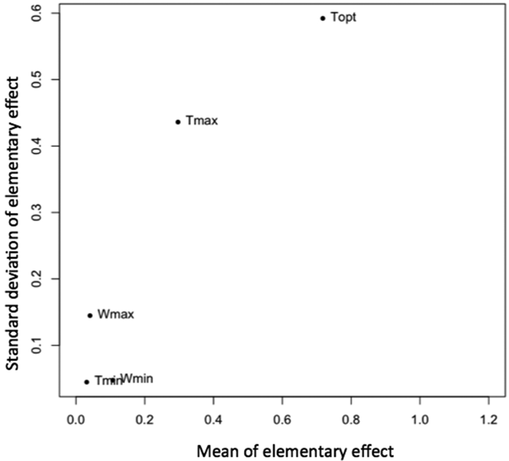
Results of the Morris method.
Five rules are presented below to improve the reliability of uncertainty and sensitivity analysis.
In some cases, conclusions of UA and SA depend on assumptions made on probability distributions of uncertain model inputs. Results may also depend on the selected method used to perform UA or SA. Ranking of parameters obtained by SA may thus depend on the method used to compute sensitivity indices. For these reasons, it is important to be transparent about assumptions made on probability distributions and to present in detail the methods used for UA/SA.
Figures 1–3 show that the uncertainty range depends highly on the temperature T. In this example, the uncertainty level can be considered as very low or very high depending on the model output; simulated wetness duration requirements were characterized by low uncertainty levels for temperatures around 27°C but by high uncertainty levels for more extreme temperatures. This example shows that the conclusions obtained for a given output may not be valid for others.
The accuracy of the estimated mean, variance, and quantiles of the probability distribution of the model output depends on the number of simulations. Figure 4 shows the 99%, 90%, 50%, 10%, and 1% percentiles of wetness duration requirements estimated using different numbers of simulations from 10 to 2 000 for T=25 °C. Estimates of the 99% percentiles of model output W were highly unstable when the number of simulations was lower than 500. In this example, at least 1 000 simulations were required to obtain accurate estimate of the 99% percentile. This result shows that it is important to check that a sufficiently high number of simulations were used in all analysis. The stability of the computed quantities can be assessed either graphically, or by computing variances, confidence intervals either analytically or by using nonparametric techniques (e.g., bootstrapping) (
Another important point to keep in mind is that results of uncertainty analysis may depend on distribution assumptions. Table 2 shows the values of the median, 95% and 99% percentiles obtained with N=10 000 Monte Carlo simulations for T=25 °C using the three different types of probability distributions described above. The 99% percentiles obtained with the three distributions were quite different. The 99% percentile was equal to 39.61 h with independent uniform distributions, but the same percentile was lower with the two other distributions, especially with distribution ii. This example illustrates the importance of assessing the robustness of results to assumptions made on probability distributions. The first step of the uncertainty analysis method specified above (Step 1: Define probability distributions for the uncertain model inputs and parameters) is a key step, and it is important to use all available information to derive reliable probability distributions reflecting correctly the current state of knowledge. Although this step is often difficult, the recent development of methods of expert elicitation and of Bayesian techniques offer new possibilities (
Estimated median, 95%, and 99% percentiles of wetness duration requirements (hours) obtained under three different assumptions of probability distributions (N=10, 000)
| Prob. distribution | Median | 95% | 99% |
|---|---|---|---|
| i. Uniform | 14.52 | 27.75 | 39.61 |
| ii. Triangular | 14.51 | 20.82 | 26.20 |
| iii. Triangular + correlation | 14.44 | 23.35 | 32.38 |
As mentioned above, several methods are available for uncertainty analysis and, even more, for sensitivity analysis. All methods do not have the same capabilities. For example, the Morris method illustrated in Figure 4 is an SA method that can be used to screen quickly among all uncertain inputs. However, this method cannot be used to distinguish between interaction and nonlinear effects, and other techniques for example Fourier amplitude sensitivity testing (FAST) and ANOVA should be applied when a precise analysis of interactions between model inputs is required.
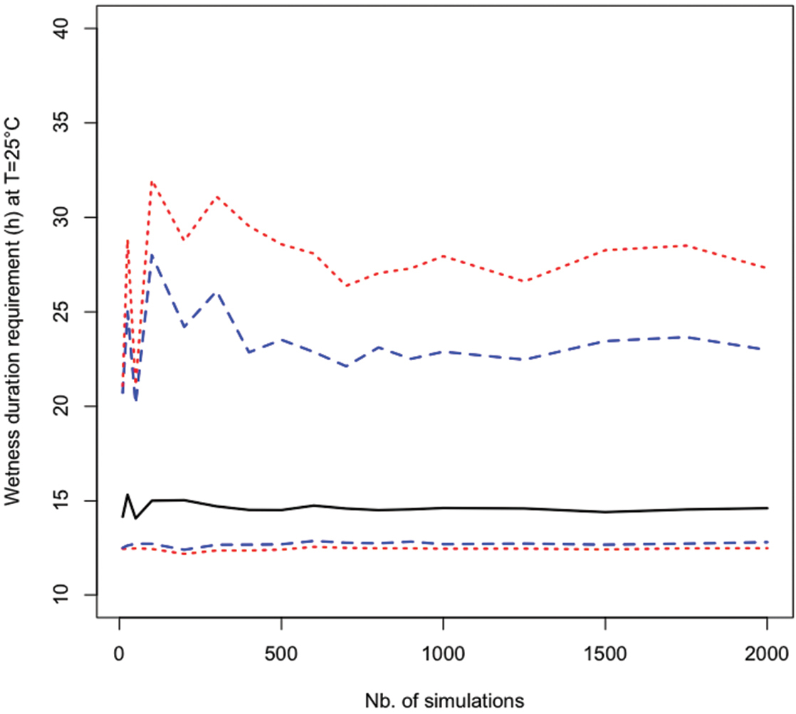
Estimated values of median (continuous line), 5% and 95% percentiles (dashed lines), 1% and 99% percentiles (dotted lines) of wetness duration requirements in function of the number of Monte Carlo simulations.
This paper shows that several factors may influence the results of uncertainty and sensitivity analysis, especially the assumptions made about the probability distributions of the uncertain model inputs and parameters, the number of simulations performed with the model, and the type of model output analyzed by the risk assessor. Due to the influence of each of these factors, the validity of the conclusions of an uncertainty or sensitivity analysis may be limited. Practical rules were presented and illustrated in this paper in order to improve the reliability of uncertainty and sensitivity analyses.