Introduction
Global tourism, trade and climate change continue to drive invasive species impact by increasing opportunities for species dispersal and establishment in new regions of the world. Nonindigenous invertebrates, vertebrates, plants, bacteria, fungi and viruses continue to establish in regions where they are not normally found (Vitousek et al. 1997), threatening both cultivated and indigenous species. Invasive species are capable of doing irreparable damage to the biodiversity of natural and agricultural ecosystems and to human and animal health, but for many nations, protecting the biological potential and production of managed systems is of particular concern, as well as increasingly urgent, as climate change threatens global food security. For greater preparedness and prevention, important decisions about invasive species need to be supported by a range of approaches that are integrative and capable of converting scientifically relevant data into data that is also decision relevant.
Regulators and pest risk assessors face the unenviable task of providing pest lists to policy makers based on their assessment of risk of pest establishment in endangered areas. When creating such lists it is difficult to ignore species that have a recent history of invasiveness. The result can be compilations that are often qualitative, subjective and frequently biased toward current knowledge and expertise of the panel involved in the creation process. Despite such drawbacks, regulators use such lists to allocate scarce resources to the prevention of perceived high risk species establishing.
Many attempts have been made to address the shortcomings of pest prioritisation but few have delivered anything that approaches a rigorous quantitative process. For example, a range of tools for prioritisation can be found in plant risk management (see Skurka Darin et al. 2011 for a brief review). Very few new tools have centred on arthropod pests or plant pathogens. Trait-based categorisation of invasive pests that aspire to give some predictive capability have been attempted with little success. For example, a study by Simberloff (1989) attempted to characterise the traits that lead to successful establishment of insects. As well, Peacock and Worner (2008) compared a selection of insect species that are often intercepted at the New Zealand border that have established, with species that, despite numerous interceptions over many years, have not yet established. The latter were used as a proxy for “failed” introductions. More recently, Philibert et al. (2011) used species–level traits of forest pathogenic fungi to predict invasion success using a combination of ecological and biological traits.
However, data associated with invasive species, as for most ecological data, involve features that are complex, dynamic and nonlinear. Many conventional multivariate statistical approaches used to analyse such data often involve linear methods that are affected by noise and outliers (Chon 2011). The purpose of this study is to review the use of the co-occurrence of pest species that make up regional species assemblages or profiles for knowledge discovery. We also review the application of novel nonlinear methods such as a neural network called Kohonen self-organising map (SOM) (Kohonen 1982) and other clustering methods, to the problem of prioritising pest species by profiling pest assemblages in target regions. Additionally, future research requirements if such methods are to be used to influence policy decisions, will be highlighted.
The idea of clustering pest complexes or assemblages of species to identify donor and recipient regions in an invasive species context was described by Worner and Gevrey (2006) using a self-organising feature map. Using species assemblages as indicators of environmental conditions is not new. Assemblages of fossil organisms such as Radiolaria and Foraminifera are used in petroleum geology and oil exploration to indicate presence of fossil hydrocarbon reservoirs (Gregory et al. 2007) as well as past climates (Heiri and Lotter 2005). Species assemblages are also well used in fresh water studies and other ecosystem studies to determine changes in composition or behaviour in response to toxic substances and responses to natural and other anthropocentric changes (Chon 2011, Lek and Guégan 2000). A SOM is an artificial neural network that can detect patterns and similarity in complex data. SOMs have found application in a range of disciplines from image recognition (see Chon 2011 for a short review) to detecting shifts in climate (Schmidt et al. 2012).
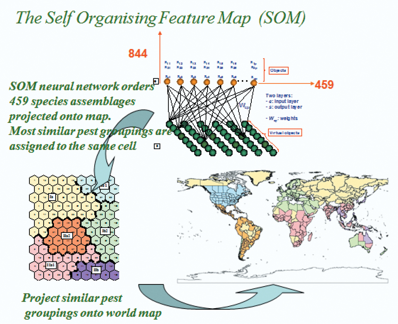
A basic assumption underpinning the Worner and Gevrey (2006) and Gevrey et al. (2006) studies is that a grouping or assemblage of pest species integrates complex variables that are difficult to tease apart. Some might question that assumption on the basis that such groupings are not natural and have come about mainly by anthropogenic influences. Despite that a history of transport, trade and food production has largely influenced which pests are where in the world, it is clear that those species able to establish viable populations rely on a complex interaction of biotic and abiotic variables. Indeed, Watts and Worner (2009a) have shown that such pest groupings are not random assemblages of species. Co-occurrence of species forming a particular pest profile for a region indicates suitable environmental conditions, and in the case of arthropod pests and plant pathogens, co-occurrence indicates suitable hosts and a particular invasion history of the region. In their 2006 study, Worner and Gevrey first used a conventional cluster analysis to identify global donor and recipient regions, using more than 800 species over 456 geopolitical areas (Worner and Gevrey 2006). The analysis resulted in long drawn out clusters that were difficult to interpret. They then applied a self-organising map (SOM) that appeared to have a number of advantages. The first is that the high dimensional data set was reduced to a 2-dimensional map or visualisation that greatly improved interpretation (Fig. 1). In addition, the analysis created a separate map for each species in the assemblage with a weight or value that indicated the strength of association that species has for the pest profiles or assemblages associated with the cells in the map. These weights allow the species complex for a region to be filtered into high risk established species and high and low risk non-established species. The high weight allocation for a species in a region indicates it is closely associated with the particular pest complex of that region. In other words, the species co-occurs globally with similar assemblages of pests. For species that are not established but allocated a high weight, the weight is interpreted as an index of high risk of establishment.
Figure 1.
A representation of the application of a self organising feature map to the analysis of pest distribution data.
Clearly, clustering can be done using a number of approaches and SOM clustering can be used in a number of contexts to address the problem of pest risk assessment. We discuss some recent studies that further explore SOM analysis or are variations of that approach, along with some alternative clustering methods in more detail.
Clustering methods and applications to risk analysis
Data
The data used in all the studies reviewed here comprised the presence and absence of pest species in different countries and regions in the world. This information was extracted with permission from the CABI Crop Protection Compendium (2003, 2007) and CABI’s Plantwise Knowledge Bank (http://www.plantwise.org/knowledgebank), which are interactive multimedia encyclopaedias edited by CABI, a not-for-profit science-based development and information organization.
Data presented by country or geographical regions where pest presence or absence is represented by binary data, with 0 corresponding to absence and 1 corresponding to presence of species in a specific geographical area. Incomplete data from the database were discarded. Depending on the taxa of interest in the study, different numbers of pest species and regions comprised the actual database used for analysis.
The SOM Model
A detailed description of self-organising maps (SOM) can be found in Kohonen (1982) and Kohonen (2001), and examples of its application to pest risk data in Worner and Gevrey (2006) as well as Gevrey et al. (2006). The self-organising map is an unsupervised learning algorithm that is a type of neural network. A SOM consists of two layers of artificial neurons, 1) the input layer that represents the input data (pest profiles comprising, presence = 1 or absence = 0 for each species in each region) and the output layer or map, which is usually arranged in a two-dimensional structure (Fig. 1). Every input neuron or vector (pest profile) is connected to every output neuron (map neuron or node), and each connection has a weight attached to it. The batch SOM algorithm can be summarized as follows: (i) Initialize the values of the virtual (node) vectors (VVi, 1 ≤ i ≤c) using random values. (ii) Repeat steps (iii) to (vi) until convergence. (iii) Read all the sample vectors (SV or pest profiles) one at a time. (iv) Compute the Euclidean distance between SV and VV. (v) Assign each SV to the nearest VV according to the distance results. (vi) Modify each VV with the mean of the SV that were assigned to it (Worner and Gevrey 2006). In other words, when the input vectors (pest profiles for global sites) are presented to the SOM algorithm, random weight values are assigned to each virtual (weight) vector associated with each neuron (node) of the map. For each input vector (pest profile) the Euclidean distance between the input vector (pest profile) and the incoming weight (node or virtual) vector of each map neuron, is calculated. Each input vector is then assigned to the closest virtual vector (the winner, also known as the best matching unit (BMU)) according to the Euclidean distance. Each virtual vector is then updated during an iterative learning process, where weights are modified according to equation (1.1).
wi, j(t+1)=wi, j(t)+h(t)(xi-wi, j(t)) (1.1)
where wi, j(t) is the connection weight from input i to map neuron j at time t, xi is element i of input vector x, and h is the neighbourhood function. In other words, the neighbourhood function determines how strongly the neurons or nodes are connected to each other, as defined in equation (2).
h(t)= α exp(-d2/(2σ2(t))) (1.2)
where α is the learning rate, which decays towards zero as time progresses, d is the Euclidean distance between the winning unit (BMU) and the current unit j, and σ is the neighbourhood width parameter, which also decays towards zero (Watts and Worner 2009b).
Basically, the large number of data vectors, or pest profiles are sorted such that those pest profiles that are most similar are associated with a particular node, neuron or cell on the map. Additionally, pest profiles associated with cells that are close to each other are more similar than those cells that are further away. While the SOM algorithm is essentially a clustering algorithm, the detail within each cluster is very useful for questions concerning the invasive species of interest. The analysis shows similarities between pest profiles of countries and regions despite that intuitively many regions may not appear to have analogous climates and environmental conditions. Clearly, however, such similarity requires close study and indeed, if the percentage similarity between any two countries in a cluster is examined one usually finds a level of similarity that is often unexpected. Clearly, the SOM analysis is only the start of a more detailed analysis into what the clusters mean. The most important result of the SOM analysis is that the SOM weights can be used to create a risk list where the weight assigned to each species (element in the vector of species) can be used as an index of the risk of those species of establishing in the target area Gevrey et al. (2006). In this way, a subset of the original 844 species can be targeted for more in-depth risk assessment.
Sensitivity analysis of SOMS
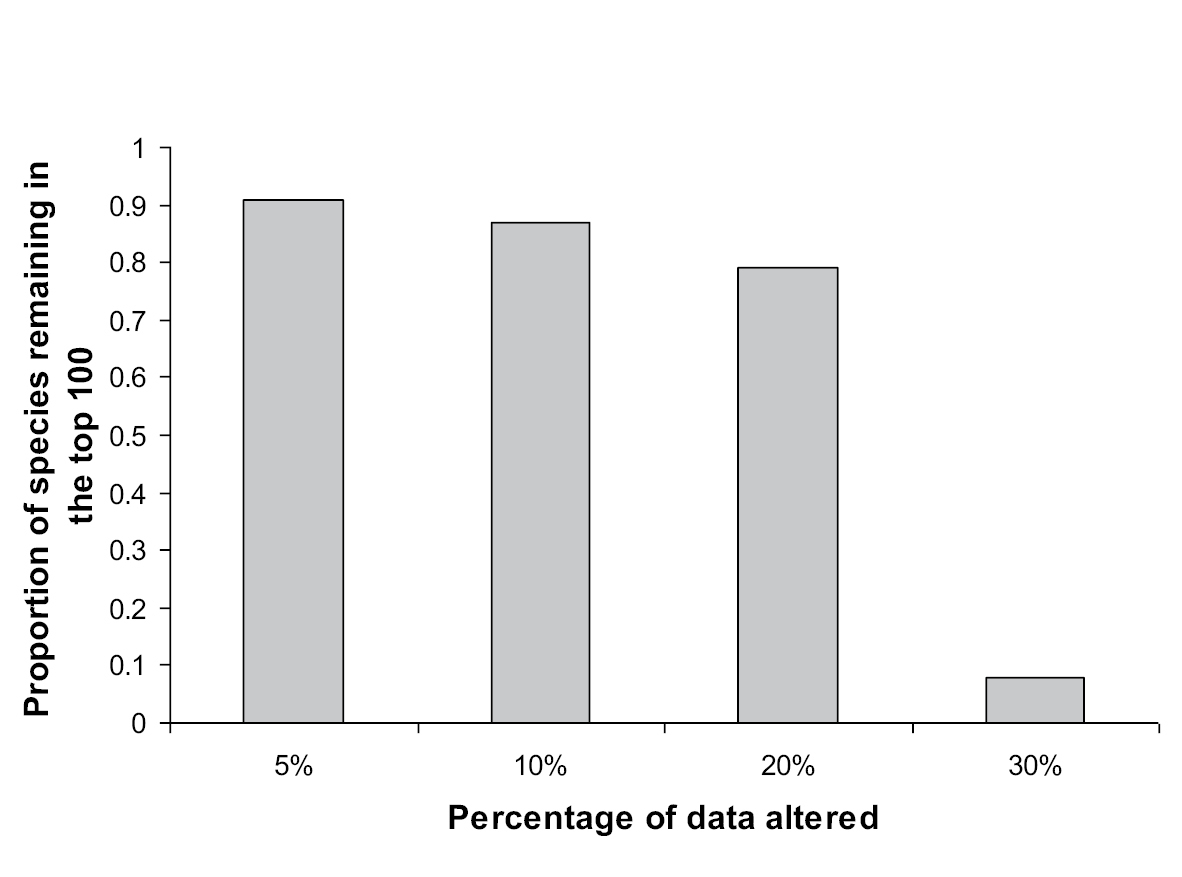
Databases often contain errors and the concern is that such error will significantly affect the confidence in any analysis that is based on the database. Paini et al. (2010a) evaluated the sensitivity of the SOM method by altering the original presence/absence data by an increasing percentage and compared estimates of risk with those generated by a national coordinating body (Plant Health Australia) utilizing expert stakeholder opinion. The same species distribution data set as used by Worner and Gevrey (2006), described above, was used in this study. Additionally, Impact Risk Assessments (IRAs) generated by the Australian Government’s Department of Agriculture, Forestry, and Fisheries (http://www.daff.gov.au/ba/ira/final-plant) were analysed to estimate the error rate in a sample of the CABI data and to determine the range of data alteration required. To simulate database error, data from all regions in the original database (459) were altered by 5%, 10%, 20%, and 30%. To do that, a set percentage of species were randomly selected from each regional pest profile and their presence or absence records reversed. Each region was altered separately so that no two regions were altered in the same way. Paini et al. (2010a) found that evaluation of the risk posed by the species based on the SOM analysis remained unaffected by alterations of up to 20% of data over all regions (Fig. 2). Of interest was the comparison of species indicated as high risk by the SOM with expert stakeholder methodology. Unsurprisingly, the comparison revealed significant differences in the estimates of establishment risk.
Figure 2.
The proportion of species remaining in the top 100 list in response to an increasing level of data alteration. (Reprinted with permission from Paini et al. 2010a).
Clearly, no data set is complete and the impact of potentially inaccurate or incomplete data was tested in another study where species profiles were bootstrapped (resampling with replacement) 1000 times and the change in each species rank (highest weight to the lowest) was recorded (Watts and Worner 2009b). The New Zealand regional pest profile was used. For the top 50 most highly ranked species, that were not established in New Zealand, their ranks changed on average only 14 places out of a possible 800, indicating considerable confidence in the method.
SOM Validation: New Zealand data
Another question is whether a SOM analysis could have helped identify those pest species that actually established in a target region. As a means of validation Worner and Soquet (2010) carried out a new SOM analysis on an updated CABI data base (CABI 2007). New Zealand’s pest profile again was used where the status of each currently established pest species was changed one at a time. In other words, if a species is established/present (1) its status was changed to not established/absent (0). The objective was to determine whether changing a species status from present to absent changes its risk index significantly. After the status of a single species was changed from present to absent, a new self-organizing map was created using the modified data and the new risk index for the target species recorded. Following that, the species status was reinstated to its original before repeating the process with the next established/present species.
By using the same initial parameters for a SOM (map size, initial weight values, number of epochs), the same clusters were formed and for each trial, the same regions were associated with the same neuron or node (cell on the map).
A rank was also associated with each species depending on its weight or risk value. Before validation the species were sorted in descending order from the species with the highest risk allocated the first rank and so on. Using ranks is a good way to measure the change in the risk by evaluating the change of rank before and after alteration. If a species rank hardly changes, in other words, if a previously present species that is changed to absent, maintains a high rank or risk index on re-analysis of the data then the self-organizing map has performed well.
The Spearman’s rank correlation between ranks obtained before and after data modification was r = 0.987, showing high correlation. Altering the data did not have a significant influence on risk assessment. A species that is highly ranked remains highly ranked even though its status is changed. Notably, the cluster to which New Zealand was assigned also never changed, nor were the adjacent neurons modified. Those results once again, illustrated the stability of the method.
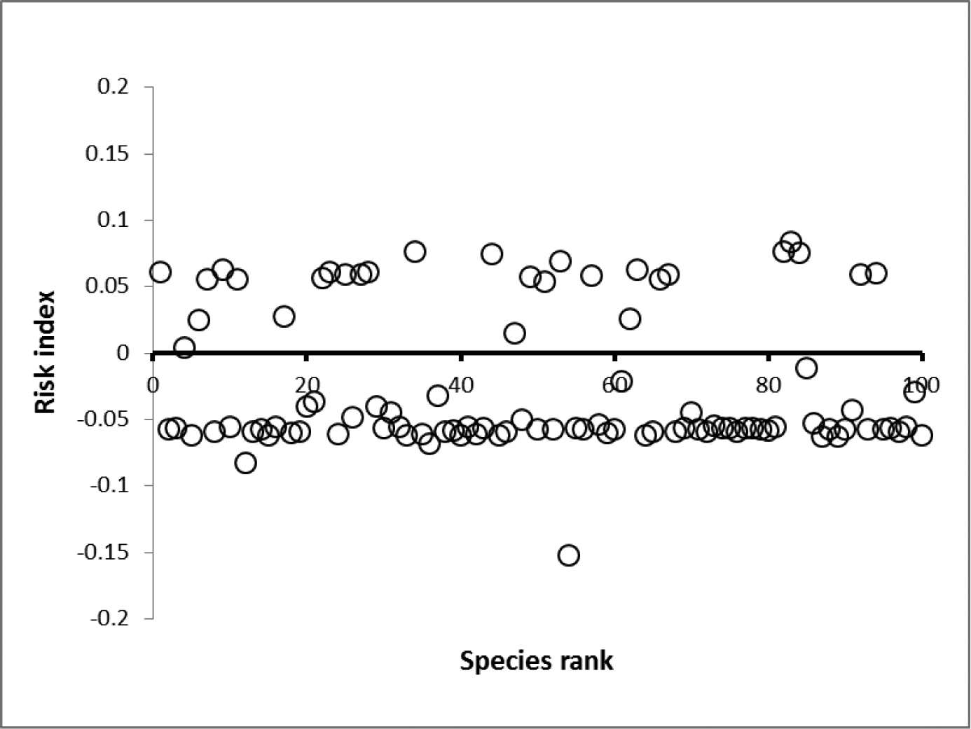
The average change in risk values for the top 100 pests was 0.07 and the ranks changed on average, 14 places (Fig. 2) for the 120 established species when their status was changed to absent (Worner and Soquet 2010). Clearly, their initial high risk index barely changed after data transformation thus a SOM analysis would have identified these species as high risk before they established in New Zealand. Despite this, a change of status of 4 of the 120 species currently present in New Zealand resulted in a change of cluster. For these 4 species the risks values also changed considerably. Some species have low initial risk simply because of low prevalence. Any interpretation of risk for low prevalence species, in other words less than about 20 occurrences, requires much caution and should be based on additional information. It is clear however that this tool is robust enough to not be influenced by even quite large variations for a large number of known global crop pests.
SOM Validation: USA data
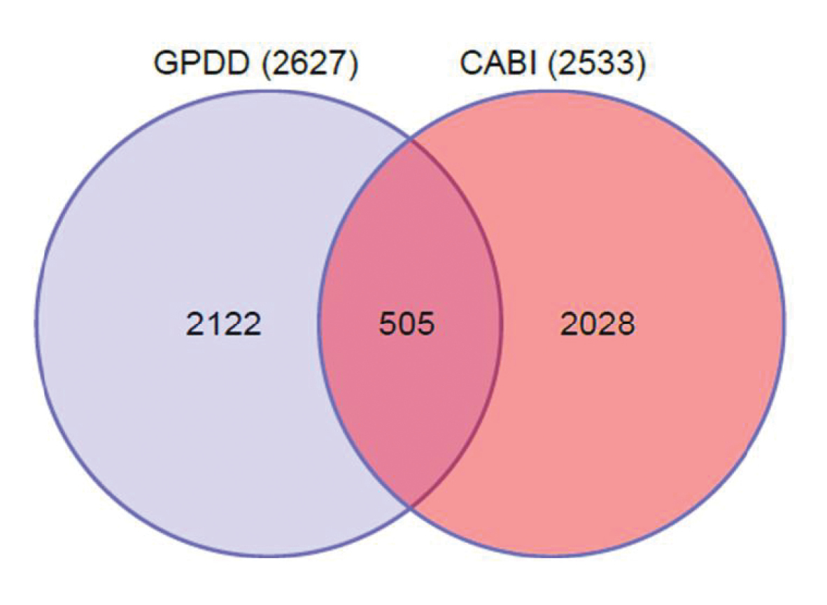
Suiter (2011) carried out a SOM analysis on USA data. The data bases used were the Global Pest and Disease Database (GPDD) which is an archive of information for pests of concern to the USA. The study also used data extracted from the CABI Crop Protection Compendium (CPC) as described above for comparative analysis. The GPDD comprised over 3000 species and is well used by many agencies such as the United States Department of Agriculture (USDA), Customs and Border Protection (CBP), Department of Homeland Security (DHS) and State Co-operators. In contrast to the study carried out by Worner and Gevrey (2006) and Gevrey et al. (2006), Suiter (2011) included all pest species recorded in the respective data bases, from bacteria to weeds, in the analysis. World pest distribution data extracted from both databases included only distributions marked as “Present”. “Unverified, Uncertain, Eradicated, Intercepted” and “Questionable” citations were discarded. The resulting analysis of the GPDD data comprised 45, 051 unique distribution records and for the CABI database, there were 47, 411 unique distribution records. Interestingly, there was only 9.8% overlap in the species recorded in each database (Fig. 4). Of particular interest with respect to validation of the SOM method was the number of high risk species, as determined by the SOM method, that were not established in 2007, that subsequently established by 2011. A 10 X 15 SOM map was used for the analysis and the databases were analysed separately.
Figure 3.
Average absolute change in risk index = 0.07.
Figure 4.
The level of similarity between the GPDD and CABI databases.
The analysis of the GPDD database showed six species with high risk indices that had not established in 2007 had established by 2011 and also six species with high risk indices in the CABI database. These species were not the same, so 12 high risk species have subsequently established by 2011. It is not known whether any of these species were regulated at the time or whether they were on any agency risk list. It appears that the SOM analysis is a useful filter that may alert risk assessors to potential threats that require a closer analysis.
Suiter (2011) found that the SOM analysis was quite robust and provided a consistent fit of the neural network to the pest distribution data. Suiter (2011) pointed out that the results of the analysis may be subject to data over- or under-sampling artefacts. For example, countries that have been heavily sampled for invasive pests (i.e., USA, China, Australia) consistently cluster together on the SOM neural net. Suiter (2011) concluded that this could be due to one or more of several factors, 1) a high probability of overlap in pest assemblages for countries with a large number of pests, 2) the countries are vast with a wide range of climates that may be very similar, 3) the countries with high pest numbers may be major trading partners and the similarities in current pest assemblages are most likely historical in nature due to trade and human movement, and 4) these countries have the resources and capacity to survey for invasive pests, unlike poorer countries. However, comparing the results of Suiter (2011) with the findings of Worner and Gevrey (2006) it appears that oversampling does not completely explain why some clusters occur. For example, Worner and Gevrey (2006) found that some countries (e.g., Tasmania, 63 species) in the New Zealand cluster had only half the number of species as some other countries (Canary Islands, 125) in the same cluster. Also the fact that trading history is important has always been proposed as one of the reasons why some pest assemblages are similar (Worner and Gevrey 2006, Paini et al. 2010b).
The Suiter (2011) study found that of the 2600 GPDD pests and 2500 CABI pests, only 505 (9.8%) (Fig. 4) were shared by both datasets and despite that, the GPDD and CABI geopolitical SOM projections looked very similar. When risk rankings were used to produce a prioritized pest list, the species compositions generated for the United States for both datasets were quite different. The study illustrates that the composition of the pest species complex present in a dataset and the distribution of species in the country of interest, are important. When there are many endemic pests in the data matrix for a large area like USA, the Euclidean distance values (risk ratings) for pests tend to be significantly lower in general than if the majority of species in the pest profile are not present in the country. That result highlights the need to analyse and interpret the results of each database separately and be mindful of endemic species that may have very low global prevalence and therefore tend not to co-occur with many other species. The fact that each database was able to highlight the risk of a number of species that had not established in 2007 but subsequently established by 2011 (Suiter 2011), illustrates that the information in each database, despite being different, is valid.
SOM Validation: simulated data
Paini et al. (2011) tested the ability of the SOM to rank fungal species that could establish in a region above those species that couldn’t establish according to simulated data. The authors did this in a virtual world in which regions had particular characteristics and species had particular requirements. Surprisingly, there was little or no difference between species that had low prevalence and species that were widely distributed and the success rate was above 90% for all species.
K-means clustering
K-means is an unsupervised algorithm that performs clustering (Lloyd 1982). In other words, the algorithm finds the best way to partition data into groups or clusters. The name k-means comes from the fact that the user decides how many clusters (k clusters) are necessary to partition data. The k-means algorithm proceeds as follows:
- Choose k initial centres. These centres (vectors) can be generated randomly or they can be vectors that are randomly selected from the data set.
- For each data vector (eg. regional pest profile), calculate the distance to each of the k cluster centres.
- Assign each data vector (pest profile) to its nearest cluster.
- Calculate new cluster centres, corresponding to the mean of all vectors in each cluster.
- Repeat steps 2-4 until a stopping condition is reached. This is usually when vectors no longer change the cluster they are assigned to, that is, the clusters are stable.
The approach of using k-means to analyse the regional pest profiles is the same as the self-organizing one where geographical regions are clustered together based on their pest species assemblage (pest profiles) to determine which species are more likely to establish in a new region. In k-means, the risk index of a species establishing in a specific region is assessed by its frequency of presence in the vectors/pest profiles in the cluster to which the target region has been assigned. Watts and Worner (2009a, 2009b, 2011, 2012) have reported a number of analyses of the CABI data set (2003, 2007) described above, using k-means clustering. In Watts and Worner (2009b) the results of clustering insect assemblages with SOM were compared with the results of the k-means algorithm. While that study found that in some ways k-means could be superior to SOM, several issues were left unaddressed such as the effect of noise or small random changes to the performance of each algorithm.
Watts and Worner (2012) compared the performance of SOM maps with the performance of equivalent k-means algorithms over assemblages of bacterial crop diseases and also investigated the effects of adding noise to the assemblages and measuring cluster quality. Cluster quality for each algorithm was measured using quantisation error (Hansen and Jaumard 1997), which is the mean distance between each vector and the centre of its cluster. In addition, the computational efficiency of each algorithm was also considered. While the Watts and Worner (2012) study found differences in the performance of the clustering algorithms in most instances the difference are not significant. More important, however, in this study as well as previous studies, the different algorithms give high to medium risk indices to basically the same species. For example, in the Watts and Worner (2012) study only 12 species out of the top 80 used for the comparisons, were not in both the SOM and k-means risk lists.
Hierarchical clustering
Borgatti (1994) and Hastie et al. (2009) give good explanations of hierarchical clustering as a means of classifying similar samples or objects. Given a set of N items to be clustered, the start of the hierarchical agglomerative clustering is to:
Assign each item to its own cluster. In each of the subsequent steps, two clusters are merged and a new cluster is formed until all clusters are merged into a single cluster. There are various methods to determine which clusters are merged, for example using the most similar pair of observations in two clusters (single linkage), the most dissimilar pair of observations (complete linkage) or the dissimilarity between the average of the observations in each cluster (group average; Hastie et al. 2009). The method used to merge clusters determines the size of the clusters and the relationships between them. A dendrogram provides a graphical representation of the relationship between the clustered items by plotting each merge at the similarity (distance) between the merged groups. It is important to note that, like the other clustering techniques discussed in this paper the clustering result does not imply a causal relationship and should be interpreted with caution.
An example of a hierarchical cluster analysis of the CABI data is provided by Eschen and Kenis (2012) who investigated the trade in woody plants for planting in Europe, as a major pathway for the introduction of alien forest pests and diseases. While phytosanitary inspections at the import stage are essential to prevent such introductions, Eschen and Kenis (2012) suggest they are limited and tend to target recognised pests, particular hosts and shipments that are likely to contain them. Such phytosanitary inspections tend to be biased, moreover, the identification of risk depends to some extent on expert judgement. The aim of the Eschen and Kenis (2012) analysis was to provide an objective assessment of the risk posed by individual species and identification or prediction of potential sources of invasive species based on the global distribution of known pests. Eschen and Kenis (2012) analysed distribution data (presence/absence data) obtained from CABI’s Plantwise Knowledge Bank (http://www.plantwise.org/knowledgebank) for 1009 invertebrate pests and pathogens of woody hosts in 351 global regions within 183 countries. Seven large countries were subdivided into regions. The 1009 taxa were divided into twelve groups (4 micro-organism and 8 invertebrate taxa).
Countries and regions with similar pest species assemblages were identified for each organism group using hierarchical cluster analysis and the likelihood of establishment of those species was calculated as the proportion or frequency of countries within the cluster containing EU and European Free Trade Association countries (EFTA) where each species has been recorded as present. Taxa recorded in fewer than six regions were excluded from the analysis to reduce the influence of rare species and outliers. Eschen and Kenis (2012) used Ward minimum variance method (Ward 1963) to determine which clusters were merged, as it consistently produced interpretable clusters, while other methods did not. The optimal number of clusters was determined for each of the twelve groups of taxa using the Davies-Bouldin Index, a measure based on the ratio between the variation within and between clusters (Davies and Bouldin 1979).
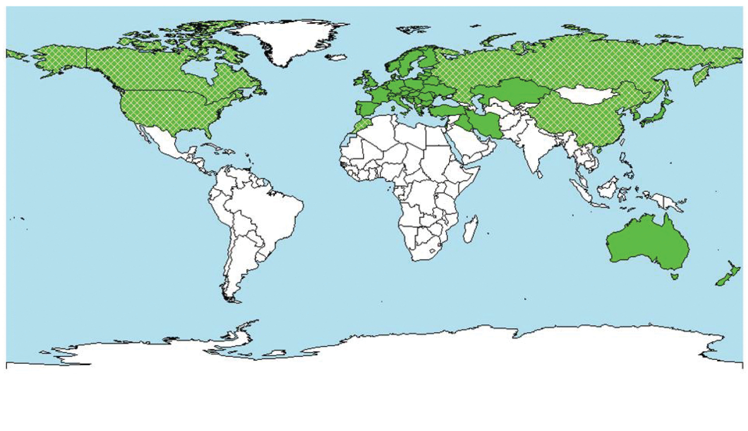
Interpretable clusters were formed for all groups of taxa, except for the Oomycetes, where the European countries were spread over all clusters. Clusters for micro-organisms contained nearly twice as many regions as clusters for invertebrates (111 vs. 61 regions per cluster). The non-EU regions with the most similar pest species assemblages to EU regions were North America, the Mediterranean region, the northern part of Eurasia and Australia/New Zealand (Fig. 5), which have a broadly similar climatic range as the EU and a long history of intensive trade. Most pest species in the database used for hierarchical analysis were already present in one or more EU countries at the time of the study, which indicated that the risk of these species primarily comes from within the EU and is similar to the result of Paini et al. (2010b), who used a SOM to identify potential new invasive agricultural invertebrate pests for the USA and also found that the majority of species in their dataset were already recorded in one or more states. Moreover, the high proportion of species already recorded in the target region lowered the risk values (Suiter 2011). Eschen and Kenis (2012) suggested that combining the results of this analysis with economic data could provide a clearer indication about the likely origin of unidentified, future alien species establishing in Europe, that should be considered when assessing the risks associated with the import of woody plants for planting.
Figure 5.
Geographical representation of the results of the hierarchical cluster analysis for species of micro-organisms and invertebrates. Countries on the map that are hatched have several regions that typically are in the European cluster. For each country and organism group, lists were produced that indicate those species that pose the greatest risk.
SOMs and multi-criteria analysis
Plant-parasitic nematodes (PPN) cause estimated losses of $157 billion/year worldwide (Abad et al. 2008) and documented losses of $600 million/year in Australia (Hodda 2009). Fortunately, Australia does not have many of the globally damaging and quarantinable PPN species and the current losses result from the activities of a relatively few damaging species, such as root-knot nematodes, root lesion nematodes, cereal cyst nematode, Heterodera avenae and potato cyst nematode, Globodera rostochiensis (in the state of Victoria only). Despite this, trade is increasing, as it is in many other countries, thus providing multiple pathways for introduction of more exotic nematode species. Based on the need for a system to prioritize risks from many PPN species and to predict their potential biosecurity threats, Singh et al. (2012) carried out a study that analysed the distribution data of 250 PPN species from 355 regions worldwide using a SOM. As in the previous studies, Singh et al. (2012) compared the presence and absence of pest species in Australia to other regions of the world by clustering regions with species assemblages similar to Australia and her component states. The SOM was also used to determine regions which could act as a donor for potential invasive species.
Singh et al. (2012) considered that in addition to distribution, there are other criteria that contribute towards the risks and impact of a species. Additionally, there are often biases in the distribution data as thorough nematode surveys are lacking in countries where there is very limited nematological expertise available. In consideration of all these factors, Singh et al. (2012) devised an assessment including the following nine criteria. For example, 1) the existence of particular pathways, 2) survival adaptations, 3) pathogenicity, 4) host range, 5) whether the species is an emerging pest, 6) its taxonomy, 7) the existence of particular pathotypes and, 8) association in disease complexes, and, 9) the level of knowledge that exists about the species. For each of the nine criteria, a probability scale was established indicating the level of risk. For example, for the pine wilt nematode, Bursaphelenchus xylophilus, and the criterion “Pathways”, they define the probability scale as, a) association with propagative material p ≥ 0.6, b) association as a contaminant, p < 0.6 > 0.3, c) not directly associated with trade p < 0.3. For each criterion, probability values were estimated based on both literature search and expert judgment. Following that, weights were assigned based on the relative contribution of each criterion towards the biosecurity risk. The SOM index from the analysis of PPN distributions was combined with the values from the nine criteria and the sum of the weighted average values was calculated to determine the overall biosecurity risk.
Initial SOM clustering indicated that potential donor regions or regions from where species are most likely to pose the greatest threat were unsurprisingly, Australia’s major trading partners. Bursaphelenchus xylophilus is a well known quarantine nematode species and based on the SOM analysis of the distribution data the resulting SOM index of 0.37 indicated the species to be of medium risk. Singh et al. (2012) used SOM index risk scale, > 0.7 = High, < 0.7 > 0.3 = Medium and < 0.3 = Low risk. When the criteria based assessment was included, the resulting risk value was much higher than that estimated by the SOM index alone (Table 1).
The higher risk is the result of considering the potential economic impacts of the species and additional information such as recent spread and availability of pathways as indicated by the number of interceptions in wood packaging materials and pine timber products. Another example is the carrot cyst nematode, Heterodera carotae, an economically important pest which currently has a restricted distribution. However, despite this restricted distribution, there is evidence of its spread and also its good survival adaptations by the formation of cysts. The SOM estimate ranked the species as low risk, but based on the multicriteria analysis, it becomes categorised as a medium risk species (Table 2).
Table 1.
SOM analysis and criteria based assessment of the pine wilt nematode (Bursaphelenchus xylophilus)
| Criteria |
Probability |
Weight |
|---|
| Distribution (SOM index from 1) |
0.37 |
0.2 |
| Pathways |
0.80 |
0.15 |
| Survival adaptations |
0.65 |
0.1 |
| Pathogenicity |
0.85 |
0.1 |
| Host range |
0.55 |
0.1 |
| Emerging pest |
0.80 |
0.1 |
| Taxonomy |
0.60 |
0.1 |
| Pathotypes |
0.50 |
0.05 |
| Disease complex |
0.60 |
0.05 |
| Knowledge |
0.45 |
0.05 |
| Sum (prob.x weight) |
|
0.62 |
Table 2.
The results of a multi-criteria analysis for a range of exotic nematode species.
| Species |
SOM Index |
Combined weighted average |
|---|
| Bursaphelenchus xylophilus |
0.37 |
0.62 |
| Heterodera carotae |
0.10 |
0.47 |
| Heterodera glycines |
0.40 |
0.63 |
| Heterodera oryzae |
0.47 |
0.52 |
| Meloidogyne chitwoodi |
0.20 |
0.62 |
The study by Singh et al. (2012) illustrates, as Worner and Gevrey (2006) suggested, that relying only on SOM estimates alone may lead to under- or overestimation of risks depending on the species. SOM remains a useful method for initial prioritization and can be incorporated with criteria based methods to better estimate a species biosecurity risks. A similar suggestion was made by Eschen and Kenis (2012), who found that their analysis did not identify Asia as a potentially important source or donor region for new invasive pests, despite a recent, strong increase in trade in plants for planting from that region.
Discussion
The studies described here suggest that SOMs can provide additional or preliminary information for evaluation and prioritisation of alien invasive species. It appears that no matter which clustering method or database is used, the analysis of similarities among pest species assemblages or regional profiles can be very useful. A criticism made by stakeholders has been that the databases used for such analyses contain a substantial number of errors. However, sensitivity analyses carried out by Paini et al. (2010a) and Watts and Worner (2009b) show that species weights and species ranks appear relatively robust to quite large errors in species distribution data. Given the many errors of omission and commission that are inevitable in such databases, these findings illustrate the practical utility of this approach and the utility of SOMs as a method, that can complement the current approaches used by biosecurity agencies. Additionally, the study by Suiter (2011) showed that quite different databases can still provide useful assessments of potential threats borne out by the number of species in each database given high risk weightings in 2007 that eventually established by 2011. In addition, the Suiter (2011) study seems to indicate that there may be some value in including other pest taxa in the analysis. The reason why the inclusion of more pest species might give better results is that more species may better characterise the pest complex by integrating more information about the abiotic and biotic influences of the region compared with fewer species. This hypothesis clearly requires more research.
With respect to the clustering methods that have been applied to the pest prioritisation problem, they all have advantages and disadvantages. The SOM analysis is computationally less efficient, but gives rich results. K-means is reputed to be susceptible to outliers and the results greatly depend on the initial partitions (the values of the cluster centres). However, an advantage of a SOM analysis is that it deals quite well with outliers. Indeed we have observed it can confine outliers in a part of the SOM map without affecting the other parts. K-means just partitions the data, whereas a SOM analysis preserves the relationship between neighbouring clusters or nodes in the map. Nearby data vectors in the input space are mapped onto neighbouring locations on the output (map) thereby preserving the internal structure of that data. SOMs also provide good data visualization and provide users with results that can simplify further analysis
Despite the difference between SOMs and k-means, a further analysis of the results in Watts and Worner (2012) shows that the differences between a k-means analysis and a SOM analysis can be minor if the same number of clusters as the SOM analysis are used. The advantage of k-means over SOM is that it is much more computationally efficient, however that does not seem so important when risk analyses, particularly when related to a new commodity or import risk assessment, may take a year or more to complete.
A striking feature when the clusters that result from the methods presented here are compared is the similarity of the results. The clusters in Worner and Gevrey (2006), Watts and Worner (2009b), Eschen and Kenis (2012) and another study by Vänninen et al. (2011) are very similar, although three techniques and two different datasets were used. The Eschen and Kenis (2012) study investigated twelve groups of invertebrates and micro-organisms with woody hosts, while the other studies investigated agricultural insect pests, but the clusters produced were strikingly similar. Such similarity suggests that the results of all three techniques were robust. However, values for the risk factors varies and a formal comparison of the methods discussed here would be desirable
Like all data analyses, the methods described here involve error. A weakness of all the clustering methods is their inability to provide a realistic risk index for species that have a restricted distribution and low prevalence, or emerging pests that initially have low prevalence and therefore low co-occurrence with other species. Although Paini et al. (2011) showed the SOM was able to successfully identify even low prevalence species as having a higher likelihood of establishing than other more widespread species that were not able to establish. The SOM method in particular identifies species that are strongly associated with a particular pest profile. For those species that are not yet established, there could be very good reasons why those species have not established but clearly they need closer study. Other information should be considered. In fact the multi-criteria analysis is a good example of first using the SOM analysis to target species for in-depth risk assessment then quantifying additional relevant information to provide a more informed risk assessment.