Sample size for inspection intended to manage risk within mixed consignments

Stephen E. Lane; Rob M. Cannon; Anthony D. Arthur; Andrew P. Robinson

doi:10.3897/neobiota.42.29757

Stephen E. Lane^‡, Rob M. Cannon^§, Anthony D. Arthur^|, Andrew P. Robinson^¶

‡ The University of Melbourne, Parkville, Australia

§ Department of Agriculture and Water Resources, Canberra, Australia

| Australian Bureau of Agricultural and Resource Economics and Sciences, Canberra, Canberra, Australia

¶ he University of Melbourne, Melbourne, Australia

Corresponding author: Stephen E. Lane ( lane.s@unimelb.edu.au )

Academic editor: Robert Colautti

This is an open access article distributed under the terms of the Creative Commons Attribution License (CC BY 4.0), which permits unrestricted use, distribution, and reproduction in any medium, provided the original author and source are credited.

Citation: Lane SE, Cannon RM, Arthur AD, Robinson AP (2019) Sample size for inspection intended to manage risk within mixed consignments. NeoBiota 42: 59-69. https://doi.org/10.3897/neobiota.42.29757

Abstract

The identification of a lot, and the size of the random sample taken for plant products, is justified by appeal to International Standards for Phytosanitary Measures No. 31, “Methodologies for Sampling of Consignments”. ISPM 31 notes that “A lot to be sampled should be a number of units of a single commodity identifiable by its homogeneity [...]” and “Treating multiple commodities as a single lot for convenience may mean that statistical inferences cannot be drawn from the results of the sampling.”

However, consignments are frequently heterogeneous, either because the same commodities have multiple sources or because there are several different commodities. The ISPM 31 prescription creates a substantial burden on border inspection because it suggests that heterogeneous populations must be split into homogeneous sub-populations from which separate samples of nominal size must be taken.

We demonstrate that if consignments with known heterogeneity are treated as stratified populations and the random sample of units is allocated proportionally based on the number of units in each stratum, then the nominal sensitivity at the consignment level is achieved if our concern is the level of contamination in the entire consignment taken as a whole. We argue that unknown heterogeneity is no impediment to appropriate statistical inference. We conclude that the international standard is unnecessarily restrictive.

Keywords

ISPM 31, stratification, biosecurity, sample-based regulatory intervention, heterogeneous population

1. Introduction

1.1 Background

Border biosecurity programs are integral to the protection of our natural environments, social amenity, and the economy through prevention of the entry of invasive pests and diseases. The economic cost (either directly, or from control measures) of invasive species has been estimated to be AUD 13.6 billion in Australia (Hoffmann and Broadhurst 2016), up to NZD 3.3 billion in New Zealand (Giera and Bell 2009), CND 34.5 billion in Canada (Colautti et al. 2006) and over USD 200 billion in the United States (Pimentel 2011).

Border inspection for biosecurity is typically the responsibility of national governments and is carried out for verifying the effectiveness of pre-arrival treatments, the detection of material that may pose a biosecurity risk, to gather information about contamination rates, and to deter any potential wrongdoing. Such pre-border and border intervention on a range of imported goods is based on the risk profile of the goods and international agreements.

It is often impractical to inspect all items in a consignment, so only a sample is inspected. In general a consignment would be deemed compliant only if no contaminated units are found in the sample, and non-compliant otherwise. For examples of sampling in the regulatory context, see Robinson (2017) and Venette et al. (2002).

The number required to be sampled is set to provide a certain probability (known as the sensitivity, or confidence level) that at least one contaminated item would be able to be detected from the sample, given a particular prevalence of contaminated items, or less often, given a specified number of contaminated items. The Binomial distribution can be used for large consignments to determine this number.

Formally, the design prevalence is denoted by p, the desired sensitivity by S_d, and the number of units to be inspected by n. The regulator sets the parameters p and S_d, then determines the number of units to be sampled (n), so that the probability that one or more contaminated units is found is greater than S_d. For large consignments we can use the Binomial distribution to obtain the sensitivity

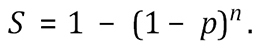(1)

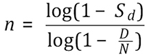
Expressing Equation (1) in terms of n gives us the (minimum) number of units to sample to achieve the desired sensitivity S_d, as:

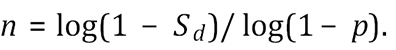(2)

2. ISPM 31 and heterogeneity

The sole statistical reference provided for the ISPM 31 sample size calculations is Cochran’s 1977 Sampling Techniques (Cochran 1977), and the calculations themselves can be located within a body of work called “design-based sampling theory”. Importantly, there is no statistical constraint or requirement for homogeneity of a sampled population within design-based sampling theory (Cochran 1977). Indeed, samples are commonly collected and analyzed across substantially heterogeneous populations, such as human and economic populations in official statistics, and forest communities in natural resource management. The only constraints are (i) that the sample be taken according to one of a number of different kinds of random sample designs, for example as detailed in ISPM 31, and (ii) if contamination is detected in any of the units sampled, then all of the lines from which samples were taken must be rejected. If the heterogeneity is unknown within a single diverse line then a simple random sample will deliver nominal sensitivity by design.

2.1 Dividing our sample between multiple lines

We now consider in detail sampling from multiple lines within a consignment. Suppose that the regulator believes it to be appropriate to sample across the K lines of a consignment as though they were a single mixed line. While we accept that each line might have a different prevalence, our criterion is that the overall prevalence in the consignment is equal to the design prevalence.

We shall find which combination of line prevalences (that satisfy the design prevalence) corresponds to the smallest overall sensitivity. By basing our calculation of the total number n of samples required on that combination of prevalences, we will ensure that the sensitivity of the inspection will be always greater than the required design sensitivity, S_d.

We shall sample a proportion w_k of the total sample from line k. Hence the sample size per line is n_k = w_kn, such that ∑_kw_k = 1. There are N_k units in the k^th line making a total of ∑_kN_k units.

If there are d_k contaminated items in line k we could use the Hypergeometric distribution to calculate the probability that none of these would be found. The result is mathematically intractable, and it is both more convenient and more conservative in regulatory contexts to use the Binomial approximation¹ based on a contamination rate expressed as a proportion of p_k = d_k / N_k. The joint contamination rate, p (our design prevalence), satisfies ∑_kN_k p_k = N.p = ∑_kd_k.

When sampling from multiple lines, the sensitivity of the inspection is of the same form as Equation (1), namely

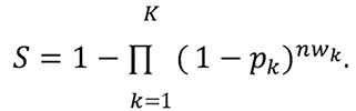(3)

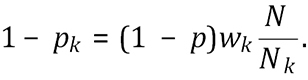Minimizing Equation (3) is equivalent to maximizing ∑_knw_klog(1 – p_k), subject to the constraint placed by the joint contamination rate, ∑_kN_k p_k = N.p. It is straightforward to show by the method of Lagrange Multipliers (Lagrange 1811) that the combination of p_k for which the sensitivity is least is:

(4)

We will now consider the optimal values for the weights w_k, beginning with the best choice, which is splitting the sample proportional to the line sizes.

2.2 Dividing the sample size proportional to the line sizes

In this section we set the sample size for each line proportional to the line size, that is w_k = N_k/N. Substituting these values into Equation (4), we find that the sensitivity will be minimized when p_k = p. Substituting these values of p_k and w_k into Equation (3), shows that the required sample size is identical to Equation (2). This choice of n and weights w_k = N_k/N ensure that the realised sensitivity will be no worse than the design sensitivity, irrespective of the individual line prevalences that satisfy the design prevalence.

The total sample size is the same as if we were sampling from a homogeneous population, as evidenced by the finding that having the same prevalence in each line corresponds to the combination of prevalences that gives the minimum sensitivity if we choose our weightings to be proportional to the line size. For any other combination of line prevalences that overall meet our design prevalence, the sensitivity of the inspection will be greater than the design sensitivity.

Figure 1 compares proportional and non-proportional allocation by way of an example; a consignment with two lines where one line has 20000 units and the other has 10000. We wish to find contamination present at the design prevalence of 0.5%, with 95% sensitivity. As already mentioned this requires a 600 unit sample (which actually corresponds to a 95.06% sensitivity). Consider three allocation schemes: the proportional allocation as just derived, requiring a sample of 400 units from the first line and 200 units from the second, and two non-proportional schemes where the sample sizes in each line are 395/205 units and 405/195 units respectively.

Figure 1.

Achieved sensitivity obtained from different allocations of the 600 units when the prevalence in each line varies so that the overall prevalence is 0.5%. The solid black line corresponding to a proportional split is always greater than the desired sensitivity. For non-proportional allocation, the sensitivity is sometimes greater and sometimes less than desired.

Figure 1 demonstrates the achieved sensitivity that would result from each allocation scheme as a function of the true contamination rate of the first line. The solid line shows the achieved sensitivity if we used proportional allocation, the horizontal line shows the nominal sensitivity, and the other lines show the two sensitivities achieved by the non-proportional allocation schemes. The key feature to note in Figure 1 is that the achieved sensitivity is always greater than the nominal sensitivity of 95% under proportional allocation, whereas it may be less under non-proportional allocations for some prevalence combinations that meet the design prevalence.

Figure 2 provides a similar comparison for a consignment of three lines for which the prevalences in the lines vary such that the overall prevalence is 0.5%. The figure shows those prevalence combinations for which the sensitivity would be less (or greater) than that desired. The left hand panel shows that the obtained sensitivity is never less than the desired sensitivity under proportional allocation. The middle and right panels are for different non-proportional division of the sample numbers: both show that there are values for which the obtained sensitivity is less than desired.

Figure 2.

Difference in achieved sensitivity under three different sampling situations. The values plotted show the regions of obtained sensitivities that are greater than or less than the desired sensitivity.

2.3 Variations of the problem

There are a number of minor variations to the problem of splitting the sample size between a number of lines. The derivations are not given but follow a similar method to the above.

2.3.1 Imperfect inspection

Sometimes our inspection will not be fully effective, and we have a probability e_k that inspection of a contaminated item in line k will detect the contamination. When our inspection method is less than perfect, we need to take more samples to compensate. It is convenient to define M_k = N_k/e_k and M = ∑_kM_k. If we divide our sample between lines according to the fraction M_k/M (rather than N_k/N), we can show that the minimum sensitivity occurs when the apparent prevalence (p_ke_k) in each line is the same by using the method in Section 2.1. From that we find that the number of samples required should be based on an adjusted (smaller) prevalence q = Np/∑_kM_k to give n = log(1–S_d)/log(1–q) and n_k = nM_k/M.

2.3.2 Design prevalence as an absolute number

Occasionally the design prevalence is specified as an absolute number D of contaminated items. Replacing p by D/N in the above gives the required sample size which, as before, would be split proportionally between the lines:

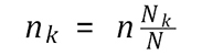
For an absolute design prevalence, log(1–D/N) needs to be calculated for each consignment. To simplify this, one can increase the sample size slightly by using the approximation log(1–D/N) ≈ –D/N (which is equivalent to using the Poisson approximation to the Binomial). The fraction

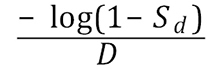
can be agreed upon by the regulator and pre-computed. This gives the overall number sampled being proportional to the number in the consignment:

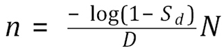2.3.3 Not knowing line sizes accurately

So far we have assumed that the counts for each line are accurately known. If the percentage errors in the counts are likely to be similar, this will be of little concern, since the relative contribution each line makes to the total will stay much the same. If, however, there is more uncertainty, the number of samples required needs to be increased for each line.

Suppose that we think the actual line sizes could be between N_k (1–α_k) and N_k (1+β_k). The consignment size would be between N (1 – α) and N (1 + β), the sum of the lower and upper line sizes respectively. Hence the weighting for line k should lie between

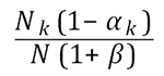and .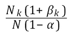

To be conservative, we use the upper limit of this range to determine the number of samples per line in terms of calculated based on Equation (2) using our desired sensitivity and design prevalence:

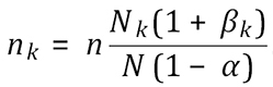Our uncertainty about line size means that we need to take more samples in total, namely

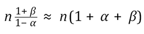As an example, if our uncertainty of the size of the consignment was of the order of ±10%, then we need to increase the sample size by approximately 20%.

2.3.4 Using fixed sample sizes

Regulators might wish to choose fixed sample sizes for each line, rather than allocate sample sizes proportional to the line sizes. For example, we could take an equal number of samples from each line. However, for such weightings, more samples are required in order to ensure the design sensitivity S_d is met. For all practical purposes, the number of samples (m) required for fixed sample sizes has to be chosen so that for each line the number of samples taken, say m_k = w_km, is greater than or equal to

the number of samples required if proportional weightings had been used.

3. Discussion and conclusions

We have shown how a standard sample size may be split between a mixed-line consignment using proportional allocation, while still at a minimum giving the desired chance of detecting contamination if it is present at a specified rate for the entire consignment. Of course, a truly random sample from the entire consignment will also give the desired sensitivity regardless of any clustering of contamination in the consignment and on average would result in a proportional number of samples being taken from each line. However, the latter approach by chance could result in no or very few samples being taken from lines with small numbers of items, something regulators might be uncomfortable with. Adopting proportional allocation would provide an explicit starting point from which samples in such lines could be increased.

If this approach to sampling is employed, it is critical for exporters to understand that if contamination is found in just one line, the entire consignment has not satisfied the import requirements and would be deemed to have failed the inspection with the resultant consequences.

The reverse is true for regulators: it is important that they do not deem only the lines in which contamination was found as non-compliant and accept the rest. The lines in which no contamination has been found have not had sufficient inspection to demonstrate that they meet the design sensitivity and prevalence requirements. Further, simply taking more samples from the ‘clean’ lines to ‘top up’ the sample size to e.g. 600 units from those lines is not enough. The actual calculation of sample sizes for such ‘topping-up’ is outside the scope of this paper. Suffice to say that the initial sample size for such a scheme must be greater than 600 units because, as well as the possibility of incorrectly accepting the consignment after the first sample, the regulator might incorrectly accept the remaining part of the consignment after the second sample.

We note that there are reasons for which processing lines separately makes operational sense. For example, the products may carry different kinds of pests that themselves present different risks, may have different levels of detection probabilities, and even different treatment possibilities. Another reason is that the exporter may not wish to take the chance that contamination in one line will affect the treatment of all of the lines in the consignment.

Our result relies on the assumption of exact proportional allocation of the samples to lines based on their counts. In some situations, the number of units in a line might differ from the nominal count, so that an exact proportional allocation would not be made. We have shown that increasing the sample size in proportion to the likely variation provides a way to ensure that the desired sensitivity is still met.

Furthermore, our result assumes that the sampling is done randomly within each line. If contamination is likely to be clustered and the sampling is not random (for example inspecting all fruit within a number of randomly-selected boxes) a different method must be used to determine the sample size (e.g. Venette et al. 2002). Extending such results from a single line is outside the scope of this paper.

Using a proportional allocation of the sample might not be prudent when the number of items in one line greatly exceeds the number in the other lines. An example of this might be with one line being melons, and one of the other lines being cherries. The problem is that proportional allocation might result in only one or two units being selected from lines with few units. While the lines with few units might only contribute a small proportion of the contamination, there may be misgivings that they haven’t been adequately inspected. One way this could be resolved is by considering them to be, from the point of view of sampling, two separate consignments. Another alternative might be to consider a box of cherries as the unit, which might give comparable unit numbers in the lines.

Another solution might be to top up the calculated number of samples to make a minimum sample per line. This would guard against missing gross contamination in a line with few units which, while not contributing greatly to the overall contamination, would be of concern if present. For example, a minimum sample of 30 in a line would detect a contamination rate of 10% in that line with a 95% probability. The other advantage in having a minimum sample size would be that information about that particular item type or source would be more quickly accumulated.

If the types of contamination in some lines are thought to have greater consequences than others, one could take extra samples above what is required in those lines, for example take twice as many. While taking extra samples is a form of non-proportional allocation, it is based on the number determined by proportional allocation: taking extra samples above the proportional allocation would increase the sensitivity of the inspection. However, to ensure the design sensitivity is met for a more general division of the sample numbers between lines (such as equally between the lines), no line should have fewer samples taken from it than the number determined by proportional allocation.

Finally, it cannot be emphasized enough: when the sample is stratified proportional to the stratum size, if contamination is found, even if it is in just one line, the whole consignment has to be deemed non-compliant and subject to whatever requirement non-compliance imposes. If this is not acceptable, then individual lines (or groups of lines) must be inspected separately, with each component subject to the specified compliance test.

1 We note that calculations based on the Hypergeometric distribution are appropriate for very small consignment sizes and/or when the inspection method is destructive and the number of samples taken needs to be minimized. In this situation it will most likely be the case that interest lies in sampling from a single line, not multiple lines as assumed in this manuscript.

References

Cochran WG (1977) Sampling Techniques (3^rd edn). John Wiley & Sons, Inc.

Colautti RI, Bailey SA, van Overdijk CDA, Amundsen K, MacIsaac HJ (2006) Characterised and Projected Costs of Nonindigenous Species in Canada. Biological Invasions 8(1): 45–59. https://doi.org/10.1007/s10530-005-0236-y

Giera N, Bell B (2009) Economic Costs of Pests to New Zealand. 2009/31. MAF Biosecurity New Zealand Technical Paper. Biosecurity New Zealand, Ministry of Agriculture; Forestry.

Hoffmann BD, Broadhurst LM (2016) The economic cost of managing invasive species in Australia. NeoBiota 31: 1–18. https://doi.org/10.3897/neobiota.31.6960

International Plant Protection Convention (2008) International standards for phytosanitary measures: ISPM 31, methodologies for sampling of consignments. Food; Agriculture Organization of the United Nations, Rome.

Lagrange J-L (1811) Mécanique Analytique. Ve Courcier, Paris.

Pimentel D (2011) Biological Invasions: Economic and Environmental Costs of Alien Plant, Animal, and Microbe Species. Second. CRC Press, Hoboken. https://doi.org/10.1201/b10938

Robinson AP (2017) Compliance and risk-based sampling for horticulture exports. 1501E, Deliverable 7. Centre of Excellence for Biosecurity Risk Analysis.

Venette RC, Moon RD, Hutchison WD (2002) Strategies and statistics of sampling for rare individuals. Annual Review of Entomology 47: 143–74. https://doi.org/10.1146/annurev.ento.47.091201.145147