Quantifying the potential impact of the European wasp (Vespula germanica) on ecosystem services in Western Australia

David C. Cook

doi:10.3897/neobiota.50.37573

Abstract

This paper estimates the ecosystem services return on investment in government control of the introduced European wasp (Vespula germanica) in the state of Western Australia. The predictive model used accounts for uncertainties in the spread and impact of V. germanica on provisioning ecosystem services, represented by pollination, apiculture and viticulture, and cultural ecosystem services represented by households. Results produced by simulating a 20-year period suggest government expenditure on management will generate net benefits of AU$3.2–6.3 million per year, most of which will accrue to producers of pollination-dependent crops. This provides justification for investment from the government’s agriculture portfolio to manage an insect often thought of as an urban pest.

Keywords

Benefit cost analysis, economic impact assessment, ecosystem service impact, European wasp, German wasp, pest management, pollination services, Vespula germanica, yellowjacket

Introduction

European wasp (Vespula germanica) is an agricultural, environmental, and urban pest first introduced to the Australian state of Western Australia (WA) in the 1970s. To support the investment of public funds on the control of this pest, this paper estimates ecosystem service benefits attributable to ongoing WA government management activities. Ecosystem services are benefits provided by ecosystems, including provisioning services like pollination and food, cultural services such as outdoor recreation, and regulating services such as flood mitigation (Costanza et al. 1997; Millennium Ecosystem Assessment 2005). This analysis focuses on avoided disruptions to provisioning services in the form of pollination, apiculture and viticulture, and cultural services in the form of household recreation.

Since the 1940s, V. germanica has spread from its native range in Europe and the Mediterranean region to North America, Chile, South Africa, New Zealand, and Australia where it has become invasive (Centre for Agricultural Bioscience Information 2017). The first detection in Australia occurred in Sydney, New South Wales in 1954 when hibernating queens were discovered on timber imported from New Zealand and destroyed (Chadwick and Nikitin 1969; Lefoe et al. 2001). The wasp then became established on the island state of Tasmania in the late 1950s (Bashford 2001). However, nests were not discovered on mainland Australia until the late 1970s (Smithers and Holloway 1977, 1978). By the early 1980s, V. germanica had spread to Victoria and South Australia (East 1984; Crosland 1991).

The first WA detection occurred in 1977 when six nests were discovered in the Freemantle port area and eradicated (Crosland 1991). Further introductions occurred in the early 1980s, and the wasp has now been reported every year since 1984 (Tennant et al. 2011). Over this period, WA’s Department of Agriculture and Food, now the Department of Primary Industries and Regional Development (DPIRD), has used targeted and passive surveillance techniques to detect and destroy wasp nests. Over 700 V. germanica nests have been destroyed across the south-west of the state, largely concentrated around the greater metropolitan Perth area (Tennant et al. 2011).

As with most government departments, DPIRD activities are highly scrutinised because of opportunity costs created with every funding decision. There is a tendency to consider state government money invested in V. germanica control as only creating social benefits in urban areas at the expense of agricultural and developmental opportunities (The Advertiser 2015; Williams 2015). While removing a public nuisance and human health concern is perceptible to the public, other more subtle benefits to pollination services, fruit growers, and beekeepers have not garnered the same amounts of attention when it comes to funding decisions. This paper shines a light on some of the less-visible benefits of V. germanica control by estimating their monetary value over time.

The premise of the paper is that without DPIRD’s activities the population of wasps and their colonies are likely to grow rapidly. Mild winter temperatures and the sandy soil of the Swan Coastal Plain on which Perth is located make the area well suited to nest building. Overwintering nests can reach large sizes by the following summer and produce thousands of new queens (Tennant et al. 2011). This would reduce pollination services to horticulture and broadacre crops as V. germanica attack wild European honeybee (Apis mellifera) hives. Attacks on managed hives will also affect apiculture, and wasps feeding on fruit will affect industries like viticulture (Clapperton et al. 1989; MacIntyre and Hellstrom 2015). These agricultural impacts are considered alongside household costs, which will rise due to the need to remove nests and avoid disruption to recreational activities.

This paper estimates the difference in ecosystem service costs under two scenarios, one in which V. germanica management in its current form is ongoing and the other in which all government efforts to manage the wasp are halted. A bioeconomic model is used to estimate damages under both scenarios over a 20-year period and, thus, damages avoided by ongoing V. germanica management. Despite being relatively simple, the model sufficies to provide indicative benefits of the management policy. Benefit estimates are then compared to the costs to government of providing management services to indicate the return on investment. All monetary values are stated in Australian dollars.

Materials and methods

Cost and revenue implications

To predict ecosystem service effects resulting from Vespula germanica spread over time under management and nil management scenarios, impacts on three provisioning ecosystem services and one cultural ecosystem service are considered.

I. Pollination impacts

Apis mellifera was introduced into Australia soon after the arrival of the first Europeans and has become widespread (Cunningham et al. 2002; Paton 1995). In WA, A. mellifera has no competitors of comparable efficiency, so insect-pollinated crops receive a high level of service from feral A. mellifera. Vespula germanica has the propensity to severely deplete honeybee colonies, placing feral or unmanaged hives at particular risk (Clapperton et al. 1989). This imposes a cost on pollinator-reliant crops, particularly horticultural crops. The crops used to predict the cost of pollination disruption from V. germanica and their pollination reliance appear in Table 1.

Table 1.

Download as

CSV

XLSX

Insect-pollinated crops in Western Australia.

Crop	Area^†(ha)	Volume^†(T)	Gross Value^‡($ million)	Pollinator reliance^§(%)
Almond	210	145	1.5	100
Avocado	8506	24621	118.4	100
Blueberry	23	81	1.8	100
Canola	1093647	1327849	730.0	15
Citrus	1436	13282	27.0	30
Cucumber	238	4028	17.8	100
Lupin	331493	457262	158.4	10
Mango	840	1424	8.1	50
Melons	591	16076	20.4	100
Pome fruit	2981	38802	98.4	50
Pumpkin	1114	18774	16.9	90
Stone fruit	298	8039	26.1	70
Strawberry	194	5112	42.5	40
TOTAL	1441571	1915495	1267.3

II. Apiculture

Managed A. mellifera hives are affected by ‘raiding’ behaviour of expanding V. germanica populations. There are approximately 28,500 managed hives in WA producing over 1,600 tonnes of honey worth $4.9 million per year (Australian Honey Bee Industry Council 2014). Beekeepers in areas where V. germanica are present must perform management actions to prevent managed hives from being destroyed. These include replenishing bee stocks that have been raided and feeding replacement bees on a sugar mixture to bring them to a productive level of health as rapidly as possible (MacIntyre and Hellstrom 2015).

III. Viticulture

Vespula germanica damage grapes and introduce foreign yeasts that can interfere with the fermentation process (Bashford 2001). Damage caused by wasps hollowing out fruit can be particularly severe, with yield losses of 10–15% having been reported in vineyards in the states of South Australia (Goodall and Smith 2001) and Victoria (Thomas 1993). In areas affected by V. germanica, additional costs are imposed on vineyard managers due to the need to bait to control wasp numbers and reduce damage to fruit.

IV. Households

Vespula germanica is a serious household pest in warmer climates where breeding and nest construction continue throughout the year, resulting in large summer colonies containing many thousands of individuals (Tennant et al. 2011). Health statistics related to wasp stings are lacking. Although no fatalities attributable to the insect reportedly occurred in the period 1979 to 1998 (McGain et al. 2000), the nuisance value associated with large colonies near homes is assumed large enough to motivate householders to invest in private pest management services in the absence of government-provided services. The cost of such services is assumed to be $200–250 per nest in the nil management scenario (FUMAPEST Pest Control 2018), and zero under the management scenario in which the WA government incurs the cost.

Uncertainty and spread prediction

Vespula germanica impacts over time are approximated using a Monte Carlo simulation model. The main purpose of the model is to provide the benefit component of a benefit cost analysis to inform DPIRD managers of likely returns to investment in V. germanica management activities. However, the model also required sufficient detail to gain traction with these managers, and to produce spread scenarios they considered plausible given their experiences with the pest.

The Monte Carlo model simulates a 20-year period. Uncertain parameters are entered as distributions and a Latin hypercube sampling algorithm used to sample from each using the @Risk software package (Palisade Software, Ithaca, New York). Parameter distribution types used in the model include: (i) PERT, a type of beta distribution specified using minimum, most likely (i.e. skewness), and maximum values; (ii) uniform, a rectangular distribution bounded by minimum and maximum values; and (iii) discrete, a distribution containing several discrete outcomes and their probabilities of occurrence. Biological and economic parameter values appear in Tables 2–5.

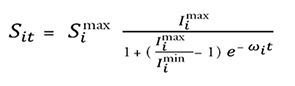
To describe changes in V. germanica impacts across multiple regions, the logistic model of Schaefer (1957) is modified to so that the length of time taken to affect horticulture pollination, apiculture, viticulture, and households can be specified. This model is combined with a measure of the marginal damage cost to simulate losses related to V. germanica over a 20-year period under nil management and management scenarios.

The model assumes that the proportion of a sector i (i.e. horticulture, apiculture, viticulture, households) affected in period t (S_it) increases over time following the logistic equation:

(1)

Here, S_i^maxis the total size of sector i affected (i.e. in number of ha for horticulture and viticulture, the number of hives for apiculture and the number of residences for households); I_i^maxis the maximum proportion of sector i affected; I_i^minis the minimum proportion of sector i affected, and; ω_i is the rate at which V. germanica moves from I_i^minto I_i^max.

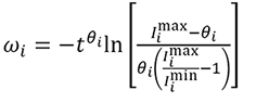
In the absence of information about ω, a hypothetical impact growth rate is used determined by the number of time periods taken for V. germanica to affect a given proportion, θ_i , of S_i^maxsuch that:

(2)

Here, θ_i is a specified proportion of S_i^maxaffected and t^θi is the number of periods (years) taken for V. germanica to reach θ_i . The values and distributions assigned to each parameter in each sector are provided in Tables 2–5.

Table 2.

Download as

CSV

XLSX

Pollination parameters.

Parameter	Nil management	Management
Biological
Infestation growth, ω_i (unitless)^†	0.33–0.83	0.22–0.33
Maximum proportion affected, I_i^max(%)^‡	Uniform(20,30)	Uniform(20,30)
Minimum proportion affected, I_i^min(%)^†	0.01	0.01
Proportion of I_i^maxaffected at t^θi , θi (%)^†	15–100	15–100
Time taken for θi to be affected (yr)^†	Uniform(10,20)	Uniform(20,30)
Economic
Demand elasticity, η^§	Uniform(−1.1,−1)	Uniform(−1.1,−1)
Discount rate, υ (%)^¶	Pert(2,5,7)	Pert(2,5,7)
Increased variable cost, V_it	0	0
Inflation rate, ι (%)^††	Pert(1.5,2,2.5)	Pert(1.5,2,2.5)
Price of per unit, P_it ($/T) ^‡‡	Almond 10300	Almond 10300
	Avocado 4800	Avocado 4800
	Blueberry 22700	Blueberry 22700
	Canola 500	Canola 500
	Citrus 2000	Citrus 2000
	Cucumber 4400	Cucumber 4400
	Lupin 300	Lupin 300
	Macadamia nut 5100	Macadamia nut 5100
	Mango 5700	Mango 5700
	Melons 1300	Melons 1300
	Pome fruit 2500	Pome fruit 2500
	Pumpkin 900	Pumpkin 900
	Stone fruit 3200	Stone fruit 3200
	Strawberry 8300	Strawberry 8300
Yield loss despite control, Y_it (%)^§§	Uniform(8,10)	Uniform(8,10)

^†See eq. A2 and explanation. The infestation growth constant ω is determined by specifying a proportion of a stock infested, θ, and the amount of time taken for this proportion to be reached (t^θ ). Assume it will take V. germanica 10–20 years to achieve an infestation rate of Uniform(10%,20%) in the nil management scenario, and 20–30 years in the management scenario. ^‡Based on pollinator reliance figures in Free (1993) and Cunningham et al. (2002). ^§ Ulubasoglu et al. (2011). ^¶ Commonwealth of Australia (2006). ^†† ABS (2018a). ^‡‡ ABS (2018b; 2018c). ^§§ Clapperton et al. (1989). New Zealand data on the percentage of hives destroyed is used as a proxy for the loss in pollination services from wild (or unmanaged) A. mellifera hives depleted by expanding V. germanica populations.

Validation of the model for all sectors in both scenarios is not possible due to a lack of data. No data exists for a nil management scenario as V. germanica has been managed since it was first detected in WA, but data relevant to the management scenario are available from DPIRD for the past 20 years (1999–2018). These data include all reported and detected instances of wasps responded to by DPIRD over time, and given the majority of activity has occurred in the Perth metropolitan area they are used as a proxy for numbers of households affected. This allowed a rudimentary validation of the model to be undertaken as it applied to the household sector using visual assessment and deviance measures.

Table 3.

Download as

CSV

XLSX

Apiculture parameters.

Parameter	Nil management	Management
Biological
Infestation growth, ω_i (unitless)^†	0.31–0.61	0.2–0.31
Maximum proportion affected, I_i^max(%)^†	Uniform(8,10)	Uniform(8,10)
Minimum proportion affected, I_i^min(%)^†	0.01	0.01
Proportion of I_i^maxaffected at t^θi , θi , (%)^†	5	5
Time taken for θi to be affected (yr)^†	Uniform(10,20)	Uniform(20,30)
Economic
Demand elasticity, η^‡	Uniform(−1.1,−1)	−0.28
Discount rate, υ (%)^§	Pert(2,5,7)	Pert(2,5,7)
Increased variable cost, V_it ($/hive)^¶	Pert(25,30,50)	Pert(25,30,50)
Inflation rate, ι (%)^††	Pert(1.5,2,2.5)	Pert(1.5,2,2.5)
Price of per unit, P_it ($/hive) ^‡‡	170	170
Yield loss despite control, Y_it (%)^¶	0–10	0–10

^†See eq. A2 and explanation. The infestation growth constant ω is determined by specifying a proportion of a stock infested, θ, and the amount of time taken for this proportion to be reached (t^θ ). The maximum proportion of hives affected is Uniform(8%, 10%) (Clapperton et al. 1989). Assume it will take V. germanica 10–20 years to achieve an infestation rate of 5% in the nil management scenario, and 20–30 years in the management scenario. ^‡ Ulubasoglu et al. (2011). ^§ Commonwealth of Australia (2006). ^¶ MacIntyre and Hellstrom (2015). Wasp management costs are based on survey response data indicating a positively skewed distribution, Pert($0,$5,$25). Bee replacement costs consist of a 1kg pack of bees plus a queen (i.e. $60) and 25 kg of sugar to build replacement bees up (i.e. $25 per hive). Yield losses are taken directly from survey response data (i.e. RiskDiscrete[(0,0.01,0.02,0.03,0.04,0.05,0.06,0.07,0.08,0.09,0.1),(0.27,0.11,0.1,0.15,0.03,0.11,0.07,0.02,0.03,0.04,0.07)]). Costs consist of (i) wasp management costs, and (ii) bee replacement costs. Monetary values have been converted to Australian dollars using an exchange rate of 0.93. ^†† ABS (2018a). ^‡‡ Australian Honey Bee Industry Council (2014).

Table 4.

Download as

CSV

XLSX

Viticulture parameters.

Parameter	Nil management	Management
Biological
Infestation growth, ω_i (unitless)^†	0.3–0.6	0.2–0.3
Maximum proportion affected, I_i^max(%)^†	Uniform(10,15)	Uniform(10,15)
Minimum proportion affected, I_i^min(%)^†	0.01	0.01
Proportion of I_i^maxaffected at t^θi , θi , (%)^†	Uniform(5,9)	Uniform(5,9)
Time taken for θi to be affected (yr)^†	Uniform(10,20)	Uniform(20,30)
Economic
Demand elasticity, η^‡	Uniform(−1.1,−1)	Uniform(−1.1,−1)
Discount rate, υ (%)^§	Pert(2,5,7)	Pert(2,5,7)
Increased variable cost, V_it ($/ha)^¶	145	145
Inflation rate, ι (%)^††	Pert(1.5,2,2.5)	Pert(1.5,2,2.5)
Price of per unit, P_it ($/T) ^‡‡	2500	2500
Yield loss despite control, Y_it (%)	0	0

^†See eq. A2 and explanation. The infestation growth constant ω is determined by specifying a proportion of a stock infested, θ, and the amount of time taken for this proportion to be reached (t^θ ). Maximum infestation of 10–15% is approximated using anecdotal information from Goodall and Smith (2001) on yield losses in South Australian vineyards. Assume it will take V. germanica 10–20 years to achieve an infestation rate of 5% in the nil management scenario, and 20–30 years in the management scenario. ^‡ Ulubasoglu et al. (2011). ^§ Commonwealth of Australia (2006). ^¶Assumes vineyard managers use baiting to control wasp numbers. Bait costs of $95 for a pack of 5 are based on Wine Tasmania (2018) and assumes bait stations are deployed at a density of 5 stations per ha per year. Assuming it takes 1 hour of labour per affected ha per year to deploy and manage bait stations, labour cost are approximately $50 per ha per year. ^†† ABS (2018a). ^‡‡ ABS (2018b) and ABS (2018c).

Visual assessment involved a graphical display of the data and model simulation output being shown to two experts involved in the DPIRD management project. They were presented with a diagram similar to Figure 1 and asked to comment on the apparent fit of the model. Both experts were reasonably comfortable that most of the data points fell within the range produced by the model and that those points that fell outside the model range were due to extenuating circumstances (i.e. chiefly the period 2003–2005 when several nests were missed, enabling a build-up that persisted over several years). However, one expert expressed concern at the upward trajectory of households affected by wasps and the negative perception on the management team’s performance.

Figure 1.

Visual validation plotting simulated and observed data of the proportion of households affected by V. germanica over the past 20 years.

Statistical validation of the model is problematic as it is stochastic, producing a distribution for comparison to each observation. Moreover, only a single set of observed time-series data is available to compare the model output against, which introduces an autocorrelation problem. As a simple deviance measure test, the mean absolute error (MAE) and mean absolute percentage error (MAPE) between observed and model output were calculated using the mean of the simulated data. The MAE was 0.14%, indicating predicted values for the proportion of households affected were an average of 0.14% from observed values. The MAPE was 8.3%, indicating prediction error is, on average, 8.3% of the observed value. As a rule of thumb, a 10% MAPE is an approximate maximum limit for model acceptance (Kleijnen 1987; Mayer and Butler 1993).

Table 5.

Download as

CSV

XLSX

Households parameters.

Parameter	Nil management	Management
Biological
Infestation growth, ω_i (unitless)^†	0.41–0.82	0.27–0.41
Maximum proportion affected, I_i^max(%)^†	1	1
Minimum proportion affected, I_i^min(%)^†	0.01	0.01
Proportion of I_i^maxaffected at t^θi , θi , (%)^†	0.9	0.9
Time taken for θi to be affected (yr)^†	Uniform(10,20)	Uniform(20,30)
Economic
Demand elasticity, η	na	na
Discount rate, υ (%)^‡	Pert(2,5,7)	Pert(2,5,7)
Increased variable cost, V_it ($/household)^§	Uniform(200,250)	Uniform(200,250)
Inflation rate, ι (%)^¶	Pert(1.5,2,2.5)	Pert(1.5,2,2.5)
Price of per unit, P_it ($/T)	na	na
Yield loss despite control, Y_it (%)	na	na

See eq. A2 and explanation. The infestation growth constant ω is determined by specifying a proportion of a stock infested, θ, and the amount of time taken for this proportion to be reached (t^θ ). Maximum infestation is approximated using data from Crosland (1991) showing the number of wasp nests destroyed in Hobart and converting this to a percentage of households using population data from McLennan (1997). Assume it will take V. germanica 10–20 years to achieve an infestation rate of 0.9% in the nil management scenario, and 20–30 years in the management scenario. The number of households in the Perth metropolitan area is assumed to be 818,100 (ABS 2017). Commercial structures are omitted. ^‡ Commonwealth of Australia (2006). ^§ FUMAPEST Pest Control (2018). ^¶ ABS (2018a).

Damage costs over time

The model estimates the ecosystem services damage (d) caused by V. germanica under nil management (d^NM) and on-going management (d^M) scenarios. The nil management scenario is constructed as a counterfactual to which a management policy can be compared to determine the reduction in damages attributable to the policy over time.

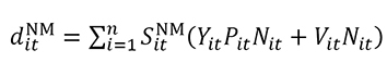
The difference between d^NMand d^Mis simulated over 20 years. The ecosystem services damage cost of V. germanica in sector i in time period t under a nil management policy (d_it^NM) is calculated as:

(3)

where: n is the number of sectors affected by V. germanica; S_it^NMis the proportion of sector i affected by V. germanica in period t under a nil management policy scenario; Y_it is the mean change in yield in sector i attributable to V. germanica in year t; P_it is the world price of product produced in sector i in year t; N_it is the number of “units” (i.e. ha, hives, residences) in sector i potentially affected by V. germanica in year t, and; V_it is the increase in variable cost per unit induced by V. germanica in sector i in year t.

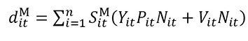
The ecosystem services damage cost of V. germanica in a region i in time period t under an ongoing management policy (d_it^NM) is calculated as:

(4)

where: S_it^Mis the proportion of sector i affected by V. germanica in period t if an ongoing management policy is in place.

For each sector that experiences yield effects from V. germanica, an estimate of price, P_it , is given for the first time step of the model (i.e. P_i0, corresponding to the year 2018). This is the initial price per unit for an affected product, but its price will change over time given that the demand for agricultural products is elastic (i.e. price increases with relative scarcity, and vice versa). The price in periods after t₀ will be partially influenced by the impact of V. germanica on production.

This price effect assumes the markets for affected products are protected, preventing perfect substitution of externally produced goods for those damaged by V. germanica. If WA markets were unregulated and open to free trade with suppliers from other states and overseas, and if the WA industries contributed a relatively small amount to global production, local prices of affected agricultural products would remain unchanged in response to V. germanica spread and impact (e.g. James and Anderson 1998). However, WA is protected by state and national phytosanitary measures and large distances separate its markets from external suppliers. Hence, reductions in local supplies tend to raise local prices.

Predicted yield loss, Y_it N_it , is used as a proxy for the V. germanica-induced reduction in sectoral output. This is combined with the lagged per unit price, P_t–1, to calculate

.

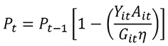Here, G_it is the gross value of production divided by 100 and η is the elasticity of demand for the affected commodity (i.e. the ratio of percentage change in quantity demanded over the percentage change in price).

Returning to equations 3 and 4, d^NMand d^Maccrue over time and are subject to discounting. Discounting has an erosive effect on monetary values that increases with time, meaning that the present value of one unit of damage caused in the present is worth more than the same amount of damage caused in the future.

Applying an exponential discount rate, the present value of benefits anticipated from an on-going management policy in time period t (PVB_t^M) is estimated by summing d_it^NM– d_it^Macross all affected sectors (n) in WA:

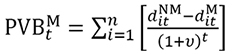(5)

where v is the discount rate.

The net present value of the V. germanica management policy (NPB_t^M) is calculated summing the difference between the present value of costs (PVC_t^M) and PVB_t^Mover m time periods:

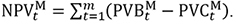(6)

The benefit cost ratio for the on-going V. germanica management option (BCR^M) is calculated by dividing the summed PVB_t^Mover m time periods by the summed PVC_t^Mover m time periods. Note that PVB_t^Mrepresents gross (as opposed to net) benefits (i.e. PVB_t^M= NPV_t^M+ PVC_t^M).

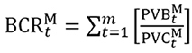. (7)

In the results section to follow, all costs and benefits are stated in Australian dollars. NPV^Mand BCR^Mare given for a range of PVC^Mbetween $230,000 and $250,000 per annum over a period of 20 years. This range approximates the total amount spent by DPIRD in the past several years, and is indexed to the inflation rate. This means that PVC^Mis fixed in real terms and nominal costs (C^M) increase at the inflation rate (ι) over time (i.e.) .

Results

Ecosystem services damage predicted by the model under the nil management scenario (i.e. d^NM, eq. 3) and on-going management scenario (i.e. d^M, eq. 4) for each sector are shown in the box-whisker plots in panels A–D of Figure 2, while panel D shows aggregated ecosystem service damages under both scenarios. In each panel, damages over time under the nil management scenario increase initially as Vespula germanica spreads, but then begin to decrease due to the effects of discounting (Epanchin-Niell and Liebhold 2015). Noting the scale differences in the y-axes of panels A–D, the largest component of damages under the nil management scenario in panel E is pollination impacts, accounting for approximately 85% in each year simulated. Household damages in panel D, attributable to necessary purchases of pest removal services, are also substantial, making up approximately 13% of total. Household damages under the management scenario are zero as nest destruction costs are paid by DPIRD.

Figure 2.

Predicted damage cost per year associated with V. germanica impacts in WA over 20 years. Panels A, B, C and D show pollination, apiculture, viticulture and household damage costs, respectively, under both scenarios, while panel E shows the summed damage costs across all sectors under both scenarios. Box whisker plots indicate 5^th, 25^th, mean, 75^thand 95^thpercentile values, with shaded boxes representing the nil management scenario and hollow boxes the management scenario.

The uncertainty in model predictions is evident in the width of the boxes and length of whiskers in Figure 2. Aggregated damage costs in panel D peak in year 12 under the nil management scenario with a mean value of $6.9 million, but vary between $5.0–9.0 million in 80% of model iterations, and between $4.6–9.7 in 90% of iterations. The present value of benefit created by DPIRD management efforts is represented by the vertical distance between the two scenarios, which in year 12 is estimated to be between $4.9–8.8 million (80%) and $4.5–9.5 million (90%).

The benefits and costs of V. germanica management are compared in Figure 3 where hollow boxes represent the present value of benefit (i.e. PVB^M, eq. 5), filled boxes represent net present value (i.e. NPV^M) and bold horizontal lines indicate the present value of costs (i.e. PVC^M). The mean annual present value of benefit and net present value between years 1–10 is $3.7 million (S.D. $1.4 million) and $3.4 million (S.D. $1.4 million), respectively. Between years 1–20, the mean present value of benefit and net present value increase to $4.9 million (S.D. $1.2 million) and $4.6 million (S.D. $1.2 million), respectively. This results in a benefit cost ratio for the management of V. germanica (i.e. BCR^M, eq. 7) over 10 years of 15.4, and over 20 years of 19.9. Based on the mean present value of benefit, the results imply each dollar invested in ongoing V. germanica management is most likely to prevent $19.90 in damage costs over 20 years.

Figure 3.

Net present value of V. germanica management in WA over 20 years. The box whisker plot indicates 5^th, 25^th, mean, 75^thand 95^thpercentile values.

However, there is considerable uncertainty in the model predictions that could lead to a substantially better or worse return on investment than indicated by the mean. Over 10 years, 80% of model iterations produced a present value of benefit of $2.1–5.6 million, suggesting a benefit cost ratio between 8.3 and 22.5. Morover, the uncertainty in model predictions increases as the length of the simulation period increases. Over 20 years, the estimated present value of benefit varies between $6.5–26.2 million, resulting in a benefit cost ratio between 13.8–26.2.

Despite this uncertainty, results of a parameter sensitivity analysis indicate that the return to investment in management remain positive even under worst-case scenarios. To gauge the effect of the parameters on model output, each parameter is sampled across its specified range while holding all other parameters constant in Figure 4. Here the 10 parameters producing the most change are ranked from top to bottom according to their strength of influence on the present value of benefit generated.

Figure 4.

Sensitivity analysis illustrating how the mean net benefit of V. germanica management in WA 20 years is affected by changes in input parameters.

Results are most sensitive to changes in the discount rate, which is specified as Pert(2%,5%,7%). It is inversely related to the present value of benefit. Lowering the discount rate from its most likely value of 5% to 2% (a change of −60%) increases the present value of benefit by approximately 31% (from $4.9 million to $6.4 million), and increasing it to 7% (a change of 40%) lowers the present value of benefit by approximately 24% (to $3.7 million). Determining an appropriate discount rate is one of the most controversial and important issues in benefit cost analysis since as it has a major impact on the viability of many public projects (Abelson and Dalton 2018). Yet there is no definitive answer as to what rate should be applied in different circumstances. This is not critical here since the present value of benefits exceed the present value of costs across the range of discount rates considered (i.e. costs do not exceed $250,000 per year in real terms).

Results are also highly sensitive to the time taken for the indicative proportion θ_i to be affected under the management scenario. This is also inversely related to the present value of benefit, producing a ±24% change when increased or decreased 20% from the mean value (25 years). As it relates to the effectiveness of DPIRD activities in slowing the spread of V. germanica, the time taken for θ_i to be affected under the management scenario is a key assumption. Citing the DPIRD time series data used to validate the model, the range 20–30 years is a reasonable approximation for this parameter. Even when at 20 years, the model still produces a present value of benefit of $3.7 million.

Other parameters with relatively high sensitivities mostly relate to the pollination sector, including yield loss despite control, increase in variable costs, maximum proportion affected (I_i^max) and the indicative proportion θ_i . This reflects the large size of pollination sector impacts compared with those in the household, viticulture and apiculture sectors.

Discussion

The model used in this analysis takes into account multiple ecosystem services and conveys the uncertain future benefits of invasive species controls to decision-makers in relatively simply terms. As the impacts of invasive species change with respect to time, location, and other variables in ways that are difficult to predict, policy-makers need to be informed by predictive (ex ante) analyses that are explicit about the uncertain future effects of decisions made in the present (Regan et al. 2002). At the same time, as they are typically time-pressured, policy-makers require model outputs that condense complex spread and impact information into easily understood metrics. The model presented here adds to the literature by simultaneously fulfilling both of these requirements.

Research concerning economic impacts of invasive species has increased in recent decades, but most has involved ex post impact assessments and management evaluation (Naylor 2000; Born et al. 2005; Cook et al. 2013). Research involving predictive models has tended to rely on partial budgeting techniques or deterministic models that ignore uncertainties in species behaviour and environmental interactions (de Wit et al. 2001; MacLeod et al. 2004; Bolda et al. 2010).

Several ex ante studies have used complex, spatially explicit approaches and stochastic simulations to characterise uncertainty in spread patterns over time combining environmental variables and invasive species behaviours (Rafoss 2003; Yemshanov et al. 2009; Leung et al. 2014). Others have integrated established ecological models with economic management frameworks (Sharov and Liebhold 1998; Barbier 2001; Cacho et al. 2008; Hyder et al. 2008; Carrasco et al. 2010) or have used metapopulation models to predict future impacts (Albers et al. 2010; Sanchirico et al. 2010).

Economic modelling has seldom been used as part of an invasive species ecosystems service impact assessment. Cook et al. (2007) used a reaction diffusion model to estimate future spread and impact of varroa bee mite (Varroa destructor) on a single ecosystem service (pollination) in Australia. Other examples include several ex post studies involving the weed leafy spurge (Euphorbia esula) that have estimated impacts on provisioning and cultural services in the northern Great Plains region of the United States (Leistritz et al. 1992; Leitch et al. 1996; Leistritz et al. 2004). Changes in grazing land output were used to estimate effects on producer and local agribusiness income, and reductions in environmental output were used to estimate changes in outdoor recreation expenditures.

The future ecosystem service impact predicted in this analysis hint at large returns to investment in the ongoing management of V. germanica in WA, particularly in terms of provisioning ecosystem services to private producers of pollination-dependent crops. This justifies the WA government’s use of DPIRD resources in managing the pest rather than another department since the impacts of the wasp are mainly agricultural. Funding is relatively low (i.e. $200,000–250,000 per year) when compared to the gross value of crops affected (i.e. $1.3 billion, see Table 1), in part due to pollination benefits being historically omitted from funding decisions.

If the pollination sector is removed from the model, the household sector becomes the largest beneficiary of management activities and the 20-year benefit cost ratio falls from 13.8–26.2 to 3.0–4.3. This might suggest the state’s demand for wasp nest removal could be met by private pest controllers in the Perth metropolitan area rather than government. The main beneficiaries are spatially concentrated in this area and benefits to the apiculture and viticulture sectors are small in comparison. Hence, the positive flow-on effects beyond the household sector would be minimal.

However, if pollination services are included in policy decisions, the situation changes considerably. Beneficiaries of management are now spatially diffuse, consisting of various industry groups, community groups and institutions. This would make it logistically challenging and prohibitively costly to bring all affected parties together to negotiate wasp management plans and control targets and monitoring with private pest control operators. Therefore, government intervention is necessary to ensure an adequate level of management services are provided to all affected groups.

If cultural ecosystem service impacts of V. germanica related to biodiversity are also included in policy decisions, the need for government intervention becomes even stronger because biological diversity is a public good. Public goods are non-rivalrous in consumption (i.e. enjoyment of biodiversity by one person does not affect the quantity available for another) and have benefits that are non-exclusive (i.e. one person cannot prevent another from enjoying the benefits of biodiversity). As such, these goods cannot be provided to a socially desirable level by private providers who are unable to charge for the full benefits their services create, nor prevent people from enjoying benefits they have not paid for.

To the author’s knowledge, no research is currently available concerning the potential for V. germanica to affect biodiversity in WA, but experience elsewhere suggests damage could be considerable. For instance, the introduction of the wasp to Tasmania has resulted in severe local reductions of invertebrates (Spradbery and Maywald 1992; Potter-Craven et al. 2018). In New Zealand, prey biomass captured by V. germanica is equivalent to that of the entire insectivorous bird fauna (Harris 1991; Toft and Beggs 1995; Toft and Rees 1998; Matthews et al. 2000). Given the status of south-west WA as a biodiversity hotspot there is a pressing need to study potential impacts on species unique to the region (Myers et al. 2000).

Conclusion

The model presented in this paper estimates the return on government investment in continued V. germanica management in WA in terms of provisioning and cultural ecosystem services. Results suggest that the combined ecosystem service benefits of ongoing management over the next 20 years are likely be $3.4–6.5 million per year. With annual costs of management being $200,000–250,000, this indicates a net benefit of $3.2–6.3 million per year. The largest beneficiaries are producers of crops depended on insect pollination. These benefits have a tendency to be overlooked due to the reputation of V. germanica as an urban nuisance, rather than an agricultural pest. If pollination benefits are ignored, households are indeed the largest beneficiaries of wasp control and there may be grounds for turning management over to the private sector. However, if pollination impacts are as large as the results of this analysis suggest, negotiation costs and information constraints are likely to prevent private controllers from providing sufficient management services. If cultural service benefits of V. germanica management are also considered, such as prevented damage to unique species in the south west of WA, the case for government provision is also strengthened.

Acknowledgements

Thank you to Catherine Webb and Marc Widmer from the Department of Primary Industries and Regional Development for information generously provided. Thanks also to two anonymous reviewers for comments and suggestions that greatly improved the paper.

References

Abelson P, Dalton T (2018) Choosing the social discount rate for Australia. Australian Economic Review 51: 52–67. https://doi.org/10.1111/1467-8462.12254

ABS (2017) Census 2016 QuickStats. Australian Bureau of Statistics, Belconnen, A.C.T.

ABS (2018a) 6401.0 – Consumer Price Index, Australia, Mar 2018. Australian Bureau of Statistics, Canberra.

ABS (2018b) Agricultural Commodities, Australia, 2015–16. Australian Bureau of Statistics, Canberra.

ABS (2018c) Value of Agricultural Commodities Produced, Australia, 2015–16. Australian Bureau of Statistics, Canberra.

Albers HJ, Fischer C, Sanchirico JN (2010) Invasive species management in a spatially heterogeneous world: effects of uniform policies. Resource and Energy Economics 32: 483–499. https://doi.org/10.1016/j.reseneeco.2010.04.001

Australian Honey Bee Industry Council (2014) Submission to senate inquiry on the future of the beekeeping and pollination service industries in Australia. Australian Honey Bee Industry Council Inc. , Raceview, Queensland, 24 pp.

Barbier EB (2001) A note on the economics of biological invasions. Ecological Economics 39: 197–202. https://doi.org/10.1016/S0921-8009(01)00239-7

Bashford R (2001) The spread and impact of the introduced vespine wasps Vespula germanica (F.) and Vespula vulgaris (L.) (Hymenoptera: Vespidae: Vespinae) in Tasmania. The Australian Entomologist 28: 1.

Bolda MP, Goodhue RE, Zalom FG (2010) Spotted wing drosophila: potential economic impact of a newly established pest. Agricultural and Resource Economics Update 13: 5–8.

Born W, Rauschmayer F, Bräuer I (2005) Economic evaluation of biological invasions – a survey. Ecological Economics 55: 321–336. https://doi.org/10.1016/j.ecolecon.2005.08.014

Cacho OJ, Wise RM, Hester SM, Sinden JA (2008) Bioeconomic modeling for control of weeds in natural environments. Ecological Economics 65: 559–568. https://doi.org/10.1016/j.ecolecon.2007.08.006

Carrasco LR, Baker R, MacLeod A, Knight JD, Mumford JD (2010) Optimal and robust control of invasive alien species spreading in homogeneous landscapes. Journal of the Royal Society Interface 7: 529–540. https://doi.org/10.1098/rsif.2009.0266

Centre for Agricultural Bioscience Information (2017) Crop Protection Compendium. CAB International, Cayman Islands.

Chadwick CE, Nikitin MI (1969) Some insects and other invertebrates intercepted in quarantine in New South Wales: Part 2. Arthropoda (excluding Coleoptera), and Mollusca. Journal of the Entomological Society of Australia 6: 37–56.

Clapperton B, Alspach P, Moller H, Matheson A (1989) The impact of common and German wasps (Hymenoptera: Vespidae) on the New Zealand beekeeping industry. New Zealand Journal of Zoology 16: 325–332. https://doi.org/10.1080/03014223.1989.10422897

Commonwealth of Australia (2006) Handbook of Cost-Benefit Analysis. Department of Finance and Administration, Canberra, 180 pp.

Cook D, Liu S, Edwards J, Villalta O, Aurambout J-P, Kriticos D, Drenth A, De Barro P (2013) An assessment of the benefits of yellow Sigatoka (Mycosphaerella musicola) control in the Queensland Northern Banana Pest Quarantine Area. NeoBiota 18: 67–81. https://doi.org/10.3897/neobiota.18.3863

Cook DC, Thomas MB, Cunningham SA, Anderson DL, De Barro PJ (2007) Predicting the economic impact of an invasive species on an ecosystem service. Ecological Applications 17: 1832–1840. https://doi.org/10.1890/06-1632.1

Costanza R, D’arge R, de Groot R, Farber S, Grasso M, Hannon B, Limburg K, Naeem S, O’neill RV, Paruelo J, Raskin RG, Sutton P, van der Belt M (1997) The value of the world’s ecosystem services and natural capital. Nature 387: 253–260. https://doi.org/10.1038/387253a0

Crosland MWJ (1991) The spread of the social wasp, Vespula germanica, in Australia. New Zealand Journal of Zoology 18: 375–387. https://doi.org/10.1080/03014223.1991.10422843

Cunningham SA, FitzGibbon F, Heard TA (2002) The future of pollinators for Australian agriculture. Australian Journal of Agricultural Research 53: 893–900. https://doi.org/10.1071/AR01186

de Wit MP, Crookes DJ, Van Wilgen BW (2001) Conflicts of interest in environmental management: estimating the costs and benefits of a tree invasion. Biological Invasions 3: 167–178. https://doi.org/10.1023/A:1014563702261

East RW (1984) Biology and control of European wasps Vespula germanica in Victoria. In: Bailey P, Swincer D (Eds) Proceedings of the Fourth Australian Applied Entomological Research Conference: Pest Control: Recent Advances and Future Prospects. Department of Agriculture, South Australia, Adelaide, 21–26.

Epanchin-Niell RS, Hastings A (2010) Controlling established invaders: integrating economics and spread dynamics to determine optimal management. Ecology Letters 13: 528–541. https://doi.org/10.1111/j.1461-0248.2010.01440.x

Epanchin-Niell RS, Liebhold AM (2015) Benefits of invasion prevention: effect of time lags, spread rates, and damage persistence. Ecological Economics 116: 146–153. https://doi.org/10.1016/j.ecolecon.2015.04.014

Free JB (1993) Insect Pollination of Crops. Academic Press, London, 684 pp.

FUMAPEST Pest Control (2018) Pest Control – European Wasps – Paper Wasps. FUMAPEST Pest Control. https://www.termite.com.au/wasps-pest-control.html [Accessed on: 2018-11-13]

Goodall S, Smith DL (2001) The European wasp in metropolitan Adelaide: it’s ecology, spread and impacts. South Australian Geographical Journal 100: 25.

Harris RJ (1991) Diet of the wasps Vespula vulgaris and V. germanica in honeydew beech forest of the South Island, New Zealand. New Zealand Journal of Zoology 18: 159–169. https://doi.org/10.1080/03014223.1991.10757963

Hyder A, Leung B, Miao ZW (2008) Integrating data, biology, and decision models for invasive species management: application to leafy spurge (Euphorbia esula). Ecology and Society 13: 1–12. https://doi.org/10.5751/ES-02485-130212

James S, Anderson K (1998) On the need for more economic assessment of quarantine policies. The Australian Journal of Agricultural and Resource Economics 42: 425–444. https://doi.org/10.1111/1467-8489.00061

Kleijnen JPC (1987) Statistical Tools for Simulation Practitioners. Marcel Dekker, New York, 448 pp.

Lefoe G, Ward D, Honan P, Darby S, Butler K (2001) Minimising the impact of European wasps on the grape and wine industry. Final report to Grape and Wine Research & Development Corporation. Department of Natural Resources and Environment, Keith Turnbull Research Institute, Frankston, 38 pp.

Leistritz F, Bangsund D, Hodur N (2004) Assessing the economic impact of invasive weeds: The case of leafy spurge (Euphorbia esula). Weed Technology 18: 1392–1395. https://doi.org/10.1614/0890-037X(2004)018[1392:ATEIOI]2.0.CO;2

Leistritz FL, Thompson F, Leitch JA (1992) Economic impact of leafy spurge (Euphorbia esula) in North Dakota. Weed Science 40: 275–280. https://doi.org/10.1017/S0043174500057349

Leitch JA, Leistritz FL, Bangsund DA (1996) Economic effect of leafy spurge in the upper Great Plains: Methods, models, and results. Impact Assessment 14: 419–433. https://doi.org/10.1080/07349165.1996.9725915

Leung B, Springborn MR, Turner JA, Brockerhoff EG (2014) Pathway‐level risk analysis: the net present value of an invasive species policy in the US. Frontiers in Ecology and the Environment 12: 273–279. https://doi.org/10.1890/130311

MacIntyre P, Hellstrom J (2015) An evaluation of the costs of pest wasps (Vespula species) in New Zealand. Department of Conservation and Ministry for Primary Industries, Wellington, 44 pp.

MacLeod A, Head J, Gaunt A (2004) An assessment of the potential economic impact of Thrips palmi on horticulture in England and the significance of a successful eradication campaign. Crop Protection 23: 601–610. https://doi.org/10.1016/j.cropro.2003.11.010

Matthews RW, Goodisman MA, Austin AD, Bashford R (2000) The introduced English wasp Vespula vulgaris (L.) (Hymenoptera: Vespidae) newly recorded invading native forests in Tasmania. Australian Journal of Entomology 39: 177–179. https://doi.org/10.1046/j.1440-6055.2000.00173.x

Mayer DG, Butler DG (1993) Statistical validation. Ecological modelling 68: 21–32. https://doi.org/10.1016/0304-3800(93)90105-2

McGain F, Harrison J, Winkel KD (2000) Wasp sting mortality in Australia. Medical journal of Australia 173: 198–200.

McLennan W (1997) 4102.0 Australian Social Trends 1996. Australian Bureau of Statistics, Belconnen, ACT, 187 pp.

Millennium Ecosystem Assessment (2005) Ecosystems and Human Well-being: Health Synthesis. Island Press, Washington, DC, 53 pp.

Myers N, Mittermeier RA, Mittermeier CG, Da Fonseca GA, Kent J (2000) Biodiversity hotspots for conservation priorities. Nature 403: 853. https://doi.org/10.1038/35002501

Naylor RL (2000) The economics of alien species invasions. In: Mooney HA, Hobbs RJ (Eds) Invasive Species in a Changing World. Island Press, Washington, DC, 241–259.

Paton DC (1995) Overview of Feral and Managed Honey Bees in Australia: Distribution, Abundance, Extent of Interactions with Native Biota, Evidence of Impacts and Future Research: Report to the Australian Nature Conservation Agency. University of Adelaide, Adelaide, 74 pp.

Potter-Craven J, Kirkpatrick JB, McQuillan PB, Bell P (2018) The effects of introduced vespid wasps (Vespula germanica and V. vulgaris) on threatened native butterfly (Oreixenica ptunarra) populations in Tasmania. Journal of Insect Conservation 22: 1–12. https://doi.org/10.1007/s10841-018-0081-9

Rafoss T (2003) Spatial stochastic simulation offers potential as a quantitative method for pest risk analysis. Risk Analysis 23: 651–661. https://doi.org/10.1111/1539-6924.00344

Regan HM, Colyvan M, Burgman MA (2002) A taxonomy and treatment of uncertainty for ecology and conservation biology. Ecological applications 12: 618–628. https://doi.org/10.1890/1051-0761(2002)012[0618:ATATOU]2.0.CO;2

Sanchirico J, Albers H, Fischer C, Coleman C (2010) Spatial management of invasive species: pathways and policy options. Environmental and Resource Economics 45: 517–535. https://doi.org/10.1007/s10640-009-9326-0

Schaefer MB (1957) Some considerations of population dynamics and economics in relation to the management of the commercial marine fisheries. Journal of the Fisheries Research Board of Canada 14: 669–681. https://doi.org/10.1139/f57-025

Sharov AA, Liebhold AM (1998) Bioeconomics of managing the spread of exotic pest species with barrier zones. Ecological Applications 8: 833–845. https://doi.org/10.1890/1051-0761(1998)008[0833:BOMTSO]2.0.CO;2

Smithers CN, Holloway GA (1977) Recent specimens of Vespula (Paravespula) germanica (Fabricius) (Hymenoptera: Vespidae) taken in Sydney. The Australian Entomologist 4: 75.

Smithers CN, Holloway GA (1978) Establishment of Vespula germanica (Fabricius) (Hymenoptera: Vespidae) in New South Wales. The Australian Entomologist 5: 55.

Spradbery J, Maywald G (1992) The distribution of the European or German wasp, Vespula germanica (F) (Hymenoptera, Vespidae), in Australia – past, present and future. Australian Journal of Zoology 40: 495–510. https://doi.org/10.1071/ZO9920495

Tennant P, Davis P, Widmer M, Hood G (2011) Final Report CRC 30133: Urban surveillance for Emergency Plant Pests (EPPs). Cooperative Research Centre for National Plant Biosecurity, Canberra, 17 pp.

The Advertiser (2015) Wasp cash ‘is a waste’. The Advertiser, 1^stOctober. News Limited Australia, Adelaide, 10.

Thomas G (1993) Wineloving wasps. Australian Horticulture, September: 28–30.

Toft RJ, Beggs JR (1995) Seasonality of crane flies (Diptera: Tipulidae) in South Island beech forest in relation to the abundance of Vespula wasps (Hymenoptera: Vespidae). New Zealand Entomologist 18: 37–43. https://doi.org/10.1080/00779962.1995.9722000

Toft RJ, Rees JS (1998) Reducing predation of orb‐web spiders by controlling common wasps (Vespula vulgaris) in a New Zealand beech forest. Ecological Entomology 23: 90–95. https://doi.org/10.1046/j.1365-2311.1998.00100.x

Ulubasoglu M, Mallick D, Wadud M, Hone P, Haszler H (2011) How price affects the demand for food in Australia – an analysis of domestic demand elasticities for rural marketing and policy. Rural Industries Research and Development Corporation, Canberra, 41 pp.

Williams T (2015) Sting in the fight against wasps. The Advertiser, 29^thSeptember. News Limited, Adelaide, 6.

Wine Tasmania (2018) European Wasp Baits. http://winetasmania.com.au/products/european_wasp_baits [Accessed on: 2018-11-15]

Yemshanov D, Koch FH, McKenney DW, Downing MC, Sapio F (2009) Mapping invasive species risks with stochastic models: A cross-border United States–Canada application for Sirex noctilio Fabricius. Risk Analysis 29: 868–864. https://doi.org/10.1111/j.1539-6924.2009.01203.x